7.1 Filtering: simple averages

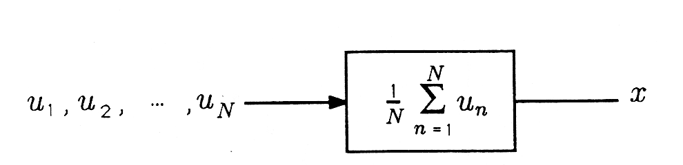
The simplest numerical filter is the simple averaging filter. This filter is defined by the equation

The filter output x is the average of the N filter inputs $u_1,u_2,...$ , u _N . These inputs may be real or complex numbers, and x may be real or complex. This simple averaging filter is illustrated in Figure 1 .

If the averaging filter is excited by the constant sequence $u_1=u_2=\cdots =u_N=u$ , then the output is

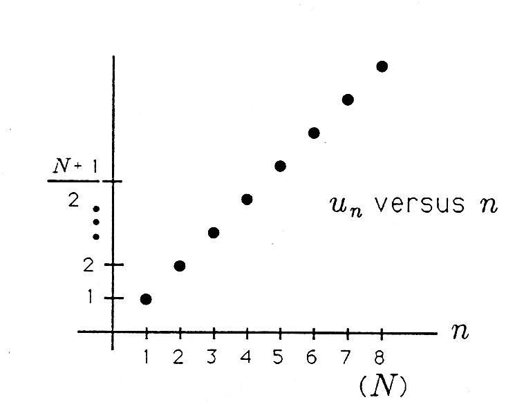
The output is, truly, the average of the inputs. Now suppose the filter is excited by the linearly increasing sequence

This sequence is plotted in Figure 2 . How do we sum such a sequence in order to produce the average $x$ ? For $N$ even, the average may be written as

Each pair-sum in parentheses equals $N+1$ , and there are $\frac{N}{2}$ such pair-sums, so the average is

This is certainly a reasonable answer for the average of a linearly increasing sequence. See Figure 2 .

General Sum Formula. Suppose the input to the simple averaging filter is the polynomial sequence

where $k$ is a non-negative integer such as $k=0,1,2,...$ . The output of the filter is

We rewrite $x$ as $x_N^{\left(k\right)}$ to remind ourselves that we are averaging $N$ numbers, each of which is $n^k$ . For example, when $N=8$ and $k=2$ ,

Rather than study the average $x_N^{\left(k\right)}$ , we will study the sum $N{x}_N^{\left(k\right)}$ and divide by $N$ at the very end:

The sum $S_N^{\left(k\right)}$ may be rewritten as the sum

This result is very important because it tells us that the sum $S_N^{\left(k\right)}$ , viewed as a function of $N$ , obeys a recursion in which $S_N^{\left(k\right)}$ is just the sum using one less input, namely, $S_{N-1}^{\left(k\right)}$ , plus $N^k$ . Now, since polynomials are the most general functions that obey such recursions, we know that $s_N^{\left(k\right)}$ must be a polynomial of order $k+1$ in the variable $N$ :

Let's check to see that this polynomial really can obey the required recursion. First note that $S_{N-1}^{\left(k\right)}$ is the following polynomial:

The term ${(N-1)}^{k+1}$ produces ${(}_0^{k+1})N^{k+1}{(-1)}^0+{(}_1^{k+1})N^k{(-1)}^1+\cdots$ . (Remember the binomial expansion?) Therefore the difference between $S_N^{\left(k\right)}$ and $S_{N-1}^{\left(k\right)}$ is

This recursion is general enough to produce the difference N ^k provided we can solve for $a_0,a_1,...$ , $a_{k+1}$ to make $c_0=c_1=\cdots =c_{k-1}=0$ and $c_k=1$ . We know that $S_N^{\left(k\right)}=0$ for $N=0$ , so we know that $a_0=0$ , meaning that the polynomial for $S_N^{\left(k\right)}$ can really be written as

In order to solve for the coefficients of this polynomial, we propose to write out our equationfor $s_N^{\left(k\right)}$ as follows:

Using the linear algebra we learned earlier, we may write these equations as the matrix equation

The terms on the right-hand side of the equal sign are “initial conditions” that tell us how the sum $S_N^{\left(k\right)}$ begins for $N=1,2,...,k+1$ . These initial conditions must be computed directly. (For example, $S_2^{\left(k\right)}=1^k+2^k.$ ) Then the linear system of $(k+1)$ equations in $(k+1)$ unknowns may be solved for $a_1,a_2,...,a_{k+1}$ . The solution for $S_N^k$ is then complete, and we may use it to solve for $S_N^k$ for arbitrary $N$ .

When $k=2$ , we have the following equation for the coefficients $a_1,a_2$ , and $a_3$ in the polynomial $S_N^{\left(2\right)}=a_{1}N+a_2{N}^2+a_3{N}^3$ :

Exponential Sums. When the input to an averaging filter is the sequence

we say that the input is exponential (or geometric). Typical sequences are illustrated in Figure 6.5 for $a=0.9,a=1$ , and $a=1.1$ . Don't let it throw you that we have changed the index to run from 0 to $N-1$ rather than from 1 to $N$ . This change is not fundamentally important, but it simplifies our study. The sum of the inputs is

How do we evaluate this sum? Well, we note that the sum $a{S}_N$ is

Therefore, provided $a\ne 1$ , the sum $S_N$ is

This formula, discovered already in the chapter covering the functions $e^x$ and $e^{j\theta }$ , works for $a\ne 1$ . When $a=1$ , then $S_N=N$ :

When $\left|a\right|<1$ , then $a^N\to 0$ for $N\to \infty$ , and we have the asymptotic formula

Recursive Computation. Every sum of the form

obeys the recursion

This means that when summing numbers you may “use them and discard them.” That is, you do not need to read them, store them, and sum them.

You may read $u_0$ to form $S_1$ and discard $u_0$ ; add $u_1$ to $S_1$ and discard $u_1$ ; add $u_2$ to $S_2$ ; and continue.

This is very important for hardware and software implementations of running sums. You need only store the current sum, not the measurements that produced it. Two illustrations of the recursion $S_{n+1}=S_n+u_n$ are provided in Figure 4 . The diagram on the left is self-explanatory. The diagram on the right says that the sum $S_n$ is stored in a memory location, to be added to $u_n$ to produce $S_{n+1}$ , which is then stored back in the memory location to be added to $u_{n+1}$ , and so on.