

| << Chapter < Page | Chapter >> Page > |
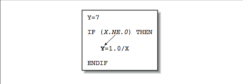

This kind of instruction scheduling will be appearing in compilers (and even hardware) more and more as time goes on. A variation on this technique is to calculate results that might be needed at times when there is a gap in the instruction stream (because of dependencies), thus using some spare cycles that might otherwise be wasted.
Expensive operation moved so that it’s rarely executed
A calculation that is in some way bound to a previous calculation is said to be data dependent upon that calculation. In the code below, the value of
B is data dependent on the value of
A . That’s because you can’t calculate
B until the value of
A is available:
A = X + Y + COS(Z)
      B = A * C
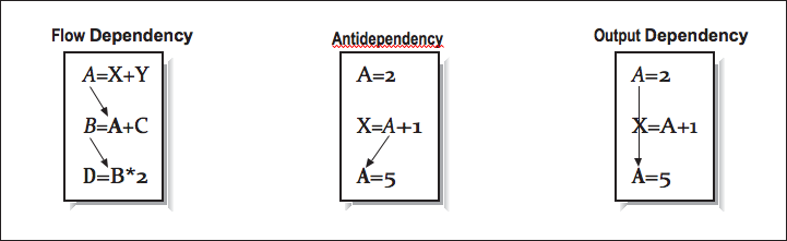
This dependency is easy to recognize, but others are not so simple. At other times, you must be careful not to rewrite a variable with a new value before every other computation has finished using the old value. We can group all data dependencies into three categories: (1) flow dependencies, (2) antidependencies, and (3) output dependencies. [link] contains some simple examples to demonstrate each type of dependency. In each example, we use an arrow that starts at the source of the dependency and ends at the statement that must be delayed by the dependency. The key problem in each of these dependencies is that the second statement can’t execute until the first has completed. Obviously in the particular output dependency example, the first computation is dead code and can be eliminated unless there is some intervening code that needs the values. There are other techniques to eliminate either output or antidependencies. The following example contains a flow dependency followed by an output dependency.
X = A / B
      Y = X + 2.0X = D - E
While we can’t eliminate the flow dependency, the output dependency can be eliminated by using a scratch variable:
Xtemp = A/B
      Y = Xtemp + 2.0X = D - E
As the number of statements and the interactions between those statements increase, we need a better way to identify and process these dependencies. [link] shows four statements with four dependencies.
Multiple dependencies
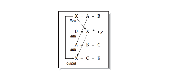
None of the second through fourth instructions can be started before the first instruction completes.
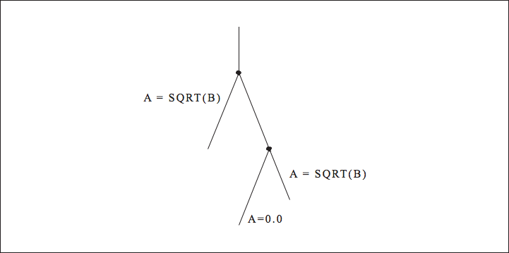
One method for analyzing a sequence of instructions is to organize it into a directed acyclic graph (DAG). A graph is a collection of nodes connected by edges. By directed, we mean that the edges can only be traversed in specified directions. The word acyclic means that there are no cycles in the graph; that is, you can’t loop anywhere within it. Like the instructions it represents, a DAG describes all of the calculations and relationships between variables. The data flow within a DAG proceeds in one direction; most often a DAG is constructed from top to bottom. Identifiers and constants are placed at the “leaf ” nodes — the ones on the top. Operations, possibly with variable names attached, make up the internal nodes. Variables appear in their final states at the bottom. The DAG’s edges order the relationships between the variables and operations within it. All data flow proceeds from top to bottom.
Notification Switch
Would you like to follow the 'High performance computing' conversation and receive update notifications?

|
|

|
|
|
|
|

|
|

|
|

|
|

|
|

|
|
|
|
|
|
|