

| << Chapter < Page | Chapter >> Page > |
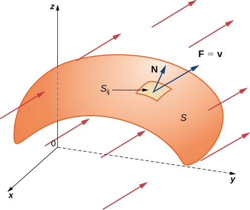
To place this definition in a real-world setting, let S be an oriented surface with unit normal vector N . Let v be a velocity field of a fluid flowing through S , and suppose the fluid has density Imagine the fluid flows through S , but S is completely permeable so that it does not impede the fluid flow ( [link] ). The mass flux of the fluid is the rate of mass flow per unit area. The mass flux is measured in mass per unit time per unit area. How could we calculate the mass flux of the fluid across S ?

The rate of flow, measured in mass per unit time per unit area, is To calculate the mass flux across S , chop S into small pieces If is small enough, then it can be approximated by a tangent plane at some point P in Therefore, the unit normal vector at P can be used to approximate across the entire piece because the normal vector to a plane does not change as we move across the plane. The component of the vector at P in the direction of N is at P . Since is small, the dot product changes very little as we vary across and therefore can be taken as approximately constant across To approximate the mass of fluid per unit time flowing across (and not just locally at point P ), we need to multiply by the area of Therefore, the mass of fluid per unit time flowing across in the direction of N can be approximated by where N , and v are all evaluated at P ( [link] ). This is analogous to the flux of two-dimensional vector field F across plane curve C , in which we approximated flux across a small piece of C with the expression To approximate the mass flux across S , form the sum As pieces get smaller, the sum gets arbitrarily close to the mass flux. Therefore, the mass flux is
This is a surface integral of a vector field. Letting the vector field be an arbitrary vector field F leads to the following definition.
Let F be a continuous vector field with a domain that contains oriented surface S with unit normal vector N . The surface integral of F over S is
Notice the parallel between this definition and the definition of vector line integral A surface integral of a vector field is defined in a similar way to a flux line integral across a curve, except the domain of integration is a surface (a two-dimensional object) rather than a curve (a one-dimensional object). Integral is called the flux of F across S , just as integral is the flux of F across curve C . A surface integral over a vector field is also called a flux integral .
Just as with vector line integrals, surface integral is easier to compute after surface S has been parameterized. Let be a parameterization of S with parameter domain D . Then, the unit normal vector is given by and, from [link] , we have
Notification Switch
Would you like to follow the 'Calculus volume 3' conversation and receive update notifications?

|
|

|
|

|
|

|
|

|
|

|
|

|
|

|
|
|
|
|

|