6.5 Vector graphics: three-dimensional homogeneous coordinates

We now consider the storage and manipulation of three-dimensional objects. We will continue to use homogeneous coordinates so that translation can be included in composite operators. Homogeneous coordinates in threedimensions will also allow us to do perspective projections so that we can view a three-dimensional object from any point in space.

Image Representation. The three-dimensional form of the point matrix in homogeneous coordinates is

The line matrix $H$ is exactly as before, pointing to pairs of columns in $G$ to connect with lines. Any other grouping matrices for objects, etc., are alsounchanged.

Image manipulations are done by a $4\times 4$ matrix A. To ensure that the fourth coordinate remains a 1, the operator A must have the structure

The new image has point matrix

Left- and Right-Handed Coordinate Systems. In this book we work exclusively with right-handed coordinate systems. However, it is worth pointing out that there are two ways to arrange the axes in three dimensions. Figure 1(a) shows the usual right-handed coordinates, and the left-handed variation is shown in Figure 1(b) . All possible choices of labels $x,y$ , and $z$ for the three coordinate axes can be rotated to fit one of these two figures, but no rotation will go from one to the other.

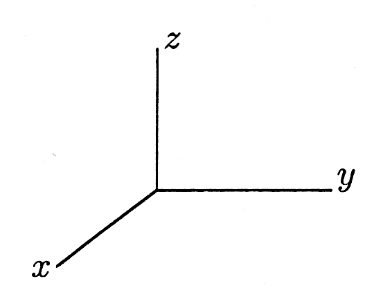
Be careful to sketch a right-handed coordinate system when you are solving problems in this chapter. Some answers will not be the same for aleft-handed system.

Image Transformation. Three-dimensional operations are a little more complicated than their two-dimensional counterparts. For scaling andtranslation we now have three independent directions, so we generalize the operators of Equation 10 from "Vector Graphics: Homogeneous Coordinates" as

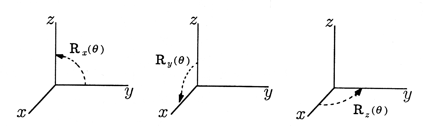
Rotation may be done about any arbitrary line in three dimensions. We will build up to the general case by first presenting the operators that rotateabout the three coordinate axes. $R_x\left(\theta \right)$ rotates by angle $\theta$ about the x-axis, with positive $\theta$ going from the y-axis to the z-axis, as shown in Figure 2 . In a similar fashion, positive rotation about the y-axis using $R_y\left(\theta \right)$ goes from $z$ to $x$ , and positive rotation about the z-axis goes from $x$ to $y$ , just as in two dimensions. We have the fundamental rotations

A more general rotation about any line through the origin can be constructed by composition of the three fundamental rotations. Finally, by composingtranslation with the fundamental rotations, we can build an operator thatrotates about any arbitrary line in space.

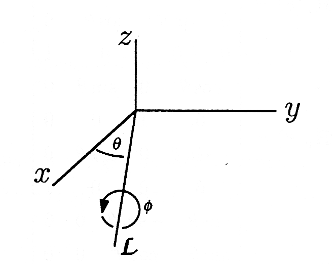
To rotate by angle $\phi$ about the line $L$ , which lies in the $x-y$ plane in Figure 3 , we would

1. rotate $L$ to the x-axis with $R_z(-\theta )$ ;
2. rotate by $\phi$ about the x-axis with $R_x\left(\phi \right)$ ; and
3. rotate back to $L$ with $R_z\left(\theta \right)$ .

The composite operation would be

Direction Cosines. As discussed in the chapter on Linear Algebra , a vector $v$ may be specified by its coordinates $(x,y,z)$ or by its length and direction. The length of $v$ is $\left|\right|v\left|\right|$ , and the direction can be specified in terms of the three direction cosines ( $cos{\theta }_x$ , $cos{\theta }_y$ , $cos{\theta }_z$ ). The angle ${\theta }_x$ is measured between the vector $v$ and the x-axis or, equivalently, between the vector $v$ and the vector $e_x=$ ${\left[100\right]}^T$ . We have

Likewise, ${\theta }_y$ is measured between $v$ and $e_y={\left[010\right]}^T$ , and ${\theta }_z$ is measured between $v$ and $e_z={\left[001\right]}^T$ . Thus

The vector

is a unit vector in the direction of $v$ , so we have

The direction cosines are useful for specifying a line in space. Instead of giving two points $P_1$ and $P_2$ on the line, we can give one point $P_1$ plus the direction cosines of any vector that points along the line. One such vector isthe vector from $P_1$ to $P_2$ .

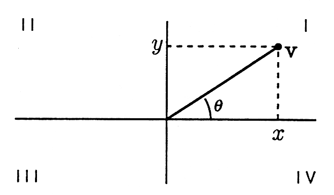
Arc tangents. Consider a vector $v=xy$ in two dimensions. We know that

for the angle $\theta$ shown in Figure 4 . If we know $x$ and $y$ , we can find $\theta$ using the arc tangent function

In MATLAB,

Unfortunately, the arc tangent always gives answers between $\frac{-\pi }{2}$ and $\frac{\pi }{2}$ corresponding to points $v$ in quadrants I and IV. The problem is that the ratio $\frac{-y}{-x}$ is the same as the ratio $---xA$ so quadrant III cannot be distinguished from quadrant I by the ratio $\frac{y}{x}$ Likewise, quadrants II and IV are indistinguishable.

The solution is the two-argument arc tangent function. In MATLAB,

will give the true angle $\theta$ $-\pi$ and $\pi$ in any of the four quadrants.

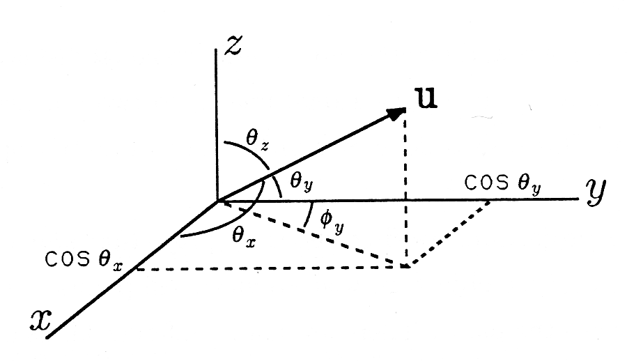
Consider the direction vector $u=cos{\theta }_{x}cos{\theta }_{y}cos{\theta }_z$ , as shown in Figure 5 . What is the angle ${\phi }_y$ between the projection of $u$ into the $x-y$ plane and the y-axis? This is important because it is $R_z\left({\phi }_y\right)$ that will put $u$ in the $y-z$ plane, and we need to know the angle ${\phi }_y$ in order to carry out this rotation. First note that it is not the same as ${\theta }_y$ . From the geometry of the figure, we can write

This gives us a formula for ${\phi }_y$ in terms of the direction cosines of $u$ . With the two-argument arc tangent, we can write