6.5 Divergence and curl  (Page 4/9)

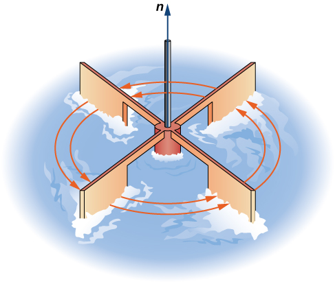
Consider the vector fields in [link] . In part (a), the vector field is constant and there is no spin at any point. Therefore, we expect the curl of the field to be zero, and this is indeed the case. Part (b) shows a rotational field, so the field has spin. In particular, if you place a paddlewheel into a field at any point so that the axis of the wheel is perpendicular to a plane, the wheel rotates counterclockwise. Therefore, we expect the curl of the field to be nonzero, and this is indeed the case (the curl is $2\text{k}).$

To see what curl is measuring globally, imagine dropping a leaf into the fluid. As the leaf moves along with the fluid flow, the curl measures the tendency of the leaf to rotate. If the curl is zero, then the leaf doesn’t rotate as it moves through the fluid.

The definition of curl can be difficult to remember. To help with remembering, we use the notation $\nabla \times \text{F}$ to stand for a “determinant” that gives the curl formula:

The determinant of this matrix is

Thus, this matrix is a way to help remember the formula for curl. Keep in mind, though, that the word determinant is used very loosely. A determinant is not really defined on a matrix with entries that are three vectors, three operators, and three functions.

If $\text{F}=⟨P,Q⟩$ is a vector field in ${ℝ}^2,$ then the curl of F , by definition, is

Finding the curl of a two-dimensional vector field

Find the curl of $\text{F}=⟨P,Q⟩=⟨y,0⟩.$

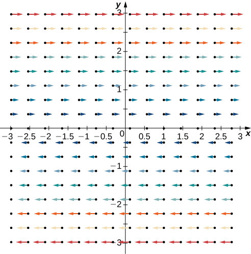
Notice that this vector field consists of vectors that are all parallel. In fact, each vector in the field is parallel to the x -axis. This fact might lead us to the conclusion that the field has no spin and that the curl is zero. To test this theory, note that

$\text{curl}\text{F}=\left(Q_x-P_y\right)\text{k}=\text{−}\text{k}\ne 0.$

Therefore, this vector field does have spin. To see why, imagine placing a paddlewheel at any point in the first quadrant ( [link] ). The larger magnitudes of the vectors at the top of the wheel cause the wheel to rotate. The wheel rotates in the clockwise (negative) direction, causing the coefficient of the curl to be negative.

Got questions? Get instant answers now!

Got questions? Get instant answers now!

Note that if $\text{F}=⟨P,Q⟩$ is a vector field in a plane, then $\text{curl}\text{F}·\text{k}=\left(Q_x-P_y\right)\text{k}·\text{k}=Q_x-P_y.$ Therefore, the circulation form of Green’s theorem is sometimes written as

where C is a simple closed curve and D is the region enclosed by C . Therefore, the circulation form of Green’s theorem can be written in terms of the curl. If we think of curl as a derivative of sorts, then Green’s theorem says that the “derivative” of F on a region can be translated into a line integral of F along the boundary of the region. This is analogous to the Fundamental Theorem of Calculus, in which the derivative of a function $f$ on line segment $[a,b]$ can be translated into a statement about $f$ on the boundary of $[a,b].$ Using curl, we can see the circulation form of Green’s theorem is a higher-dimensional analog of the Fundamental Theorem of Calculus.