

| << Chapter < Page | Chapter >> Page > |
A region D is a connected region if, for any two points and there is a path from to with a trace contained entirely inside D . A region D is a simply connected region if D is connected for any simple closed curve C that lies inside D , and curve C can be shrunk continuously to a point while staying entirely inside D . In two dimensions, a region is simply connected if it is connected and has no holes.
All simply connected regions are connected, but not all connected regions are simply connected ( [link] ).
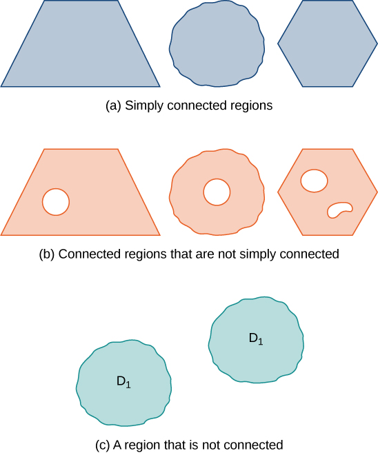
Is the region in the below image connected? Is the region simply connected?

The region in the figure is connected. The region in the figure is not simply connected.
Now that we understand some basic curves and regions, let’s generalize the Fundamental Theorem of Calculus to line integrals. Recall that the Fundamental Theorem of Calculus says that if a function has an antiderivative F , then the integral of from a to b depends only on the values of F at a and at b —that is,
If we think of the gradient as a derivative, then the same theorem holds for vector line integrals. We show how this works using a motivational example.
Let Calculate where C is the line segment from (0,0) to (2,2)( [link] ).
We use [link] to calculate Curve C can be parameterized by Then, and which implies that
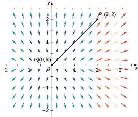
Notice that where If we think of the gradient as a derivative, then is an “antiderivative” of F . In the case of single-variable integrals, the integral of derivative is where a is the start point of the interval of integration and b is the endpoint. If vector line integrals work like single-variable integrals, then we would expect integral F to be where is the endpoint of the curve of integration and is the start point. Notice that this is the case for this example:
and
In other words, the integral of a “derivative” can be calculated by evaluating an “antiderivative” at the endpoints of the curve and subtracting, just as for single-variable integrals.
The following theorem says that, under certain conditions, what happened in the previous example holds for any gradient field. The same theorem holds for vector line integrals, which we call the Fundamental Theorem for Line Integrals.
Let C be a piecewise smooth curve with parameterization Let be a function of two or three variables with first-order partial derivatives that exist and are continuous on C . Then,
Notification Switch
Would you like to follow the 'Calculus volume 3' conversation and receive update notifications?

|
|

|
|

|
|

|
|

|
|

|
|

|
|

|
|
|
|
|
|
|