6.2 Line integrals  (Page 5/20)

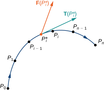
Let $\text{r}\left(t\right)$ be a parameterization of C for $a\le t\le b$ such that the curve is traversed exactly once by the particle and the particle moves in the positive direction along C . Divide the parameter interval $\left[a,b\right]$ into n subintervals $\left[t_{i-1},t_i\right],0\le i\le n,$ of equal width. Denote the endpoints of $\text{r}\left(t_0\right),\text{r}\left(t_1\right)\text{,…},\text{r}\left(t_n\right)$ by $P_0\text{,…},P_n.$ Points P _i divide C into n pieces. Denote the length of the piece from P _i−1 to P _i by $\text{Δ}{s}_i.$ For each i , choose a value $t_i^{*}$ in the subinterval $\left[t_{i-1},t_i\right].$ Then, the endpoint of $\text{r}(t_i^{*})$ is a point in the piece of C between $P_{i-1}$ and P _i ( [link] ). If $\text{Δ}{s}_i$ is small, then as the particle moves from $P_{i-1}$ to $P_i$ along C , it moves approximately in the direction of $\text{T}\left(P_i\right),$ the unit tangent vector at the endpoint of $\text{r}(t_i^{*}).$ Let $P_i^{*}$ denote the endpoint of $\text{r}(t_i^{*}).$ Then, the work done by the force vector field in moving the particle from $P_{i-1}$ to P _i is $\text{F}\left(P_i^{*}\right)·\left(\text{Δ}{s}_i\text{T}\left(P_i^{*}\right)\right),$ so the total work done along C is

Letting the arc length of the pieces of C get arbitrarily small by taking a limit as $n\to \infty$ gives us the work done by the field in moving the particle along C . Therefore, the work done by F in moving the particle in the positive direction along C is defined as

which gives us the concept of a vector line integral.

With scalar line integrals, neither the orientation nor the parameterization of the curve matters. As long as the curve is traversed exactly once by the parameterization, the value of the line integral is unchanged. With vector line integrals, the orientation of the curve does matter. If we think of the line integral as computing work, then this makes sense: if you hike up a mountain, then the gravitational force of Earth does negative work on you. If you walk down the mountain by the exact same path, then Earth’s gravitational force does positive work on you. In other words, reversing the path changes the work value from negative to positive in this case. Note that if C is an oriented curve, then we let − C represent the same curve but with opposite orientation.

As with scalar line integrals, it is easier to compute a vector line integral if we express it in terms of the parameterization function r and the variable t . To translate the integral ${\displaystyle {\int }_C\text{F}·\text{T}ds}$ in terms of t , note that unit tangent vector T along C is given by $\text{T}=\frac{r^{\prime }\left(t\right)}{\Vert r^{\prime }\left(t\right)\Vert }$ (assuming $\Vert r^{\prime }\left(t\right)\Vert \ne 0).$ Since $ds=\Vert r^{\prime }\left(t\right)\Vert dt,$ as we saw when discussing scalar line integrals, we have

Thus, we have the following formula for computing vector line integrals:

Because of [link] , we often use the notation ${\displaystyle {\int }_C\text{F}·d\text{r}}$ for the line integral ${\displaystyle {\int }_C\text{F}·\text{T}ds.}$

If $\text{r}\left(t\right)=⟨x\left(t\right),y\left(t\right),z\left(t\right)⟩,$ then d r denotes vector $⟨x^{\prime }\left(t\right),y^{\prime }\left(t\right),z^{\prime }\left(t\right)⟩.$

Evaluating a vector line integral

Find the value of integral ${\displaystyle {\int }_C\text{F}·d\text{r},}$ where $C$ is the semicircle parameterized by $\text{r}(t)=⟨\text{cos}t,\text{sin}t⟩,$ $0\le t\le \pi$ and $\text{F}=⟨\text{−}y,x⟩.$

We can use [link] to convert the variable of integration from s to t . We then have

$\text{F}(\text{r}(t))=⟨\text{−}\text{sin}t,\text{cos}t⟩\text{and}{r}^{\prime }(t)=⟨\text{−}\text{sin}t,\text{cos}t⟩.$

Therefore,

$\begin{array}{cc}\hfill {\displaystyle {\int }_C\text{F}}·d\text{r}& ={\displaystyle {\int }_0^{\pi }⟨\text{−}\text{sin}t,\text{cos}t⟩·⟨\text{−}\text{sin}t,\text{cos}t⟩dt}\hfill \\ & ={\displaystyle {\int }_0^{\pi }{\text{sin}}^{2}t}+{\text{cos}}^{2}tdt\hfill \\ & ={\displaystyle {\int }_0^{\pi }1dt}=\pi .\hfill \end{array}$

See [link] .

Got questions? Get instant answers now!

Got questions? Get instant answers now!