6.2 Line integrals  (Page 2/20)

You may have noticed a difference between this definition of a scalar line integral and a single-variable integral. In this definition, the arc lengths $\text{Δ}{s}_1,\text{Δ}{s}_2\text{,…},\text{Δ}{s}_n$ aren’t necessarily the same; in the definition of a single-variable integral, the curve in the x -axis is partitioned into pieces of equal length. This difference does not have any effect in the limit. As we shrink the arc lengths to zero, their values become close enough that any small difference becomes irrelevant.

If $f$ is a continuous function on a smooth curve C , then ${\displaystyle {\int }_{C}fds}$ always exists. Since ${\displaystyle {\int }_{C}fds}$ is defined as a limit of Riemann sums, the continuity of $f$ is enough to guarantee the existence of the limit, just as the integral ${\displaystyle {\int }_a^{b}g\left(x\right)dx}$ exists if g is continuous over $\left[a,b\right].$

Before looking at how to compute a line integral, we need to examine the geometry captured by these integrals. Suppose that $f\left(x,y\right)\ge 0$ for all points $\left(x,y\right)$ on a smooth planar curve $C.$ Imagine taking curve $C$ and projecting it “up” to the surface defined by $f\left(x,y\right),$ thereby creating a new curve $C^{\prime }$ that lies in the graph of $f\left(x,y\right)$ ( [link] ). Now we drop a “sheet” from $C^{\prime }$ down to the xy-plane. The area of this sheet is ${\displaystyle {\int }_{C}f\left(x,y\right)ds}.$ If $f\left(x,y\right)\le 0$ for some points in $C,$ then the value of ${\displaystyle {\int }_{C}f\left(x,y\right)ds}$ is the area above the xy-plane less the area below the xy-plane. (Note the similarity with integrals of the form ${\displaystyle {\int }_a^{b}g\left(x\right)dx.})$

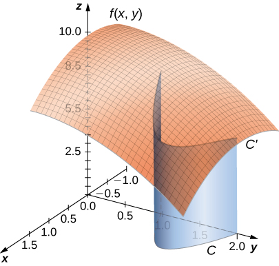
From this geometry, we can see that line integral ${\displaystyle {\int }_{C}f\left(x,y\right)ds}$ does not depend on the parameterization $\text{r}\left(t\right)$ of C . As long as the curve is traversed exactly once by the parameterization, the area of the sheet formed by the function and the curve is the same. This same kind of geometric argument can be extended to show that the line integral of a three-variable function over a curve in space does not depend on the parameterization of the curve.

Finding the value of a line integral

Find the value of integral ${\displaystyle {\int }_{C}2ds,}$ where $C$ is the upper half of the unit circle.

The integrand is $f\left(x,y\right)=2.$ [link] shows the graph of $f\left(x,y\right)=2,$ curve C , and the sheet formed by them. Notice that this sheet has the same area as a rectangle with width $\pi$ and length 2. Therefore, ${\displaystyle {\int }_{C}2ds=2\pi .}$

To see that ${\displaystyle {\int }_{C}2ds=2\pi }$ using the definition of line integral, we let $\text{r}\left(t\right)$ be a parameterization of C . Then, $f\left(\text{r}\left(t_i\right)\right)=2$ for any number $t_i$ in the domain of r . Therefore,

$\begin{array}{cc}\hfill {\displaystyle {\int }_{C}f}ds& =\underset{n\to \infty }{\text{lim}}{\displaystyle \sum _{i=1}^{n}f\left(\text{r}\left(t_i^{*}\right)\right)\text{Δ}{s}_i}\hfill \\ & =\underset{n\to \infty }{\text{lim}}{\displaystyle \sum _{i=1}^{n}2\text{Δ}{s}_i}\hfill \\ & =2\underset{n\to \infty }{\text{lim}}{\displaystyle \sum _{i=1}^{n}2\text{Δ}{s}_i}\hfill \\ & =2\left(\text{length of C}\right)\hfill \\ & =2\pi .\hfill \end{array}$

Got questions? Get instant answers now!

Got questions? Get instant answers now!