<< Chapter < Page Chapter >> Page >
I 0 Z = I 0 2 R 2 + ( I 0 X L I 0 X C ) 2 = I 0 R 2 + ( X L X C ) 2 . size 12{I rSub { size 8{0} } Z= sqrt {I rSub { size 8{0} rSup { size 8{2} } } R rSup { size 8{2} } + \( I rSub { size 8{0} } X rSub { size 8{L} } - I rSub { size 8{0} } X rSub { size 8{C} } \) rSup { size 8{2} } } =I rSub { size 8{0} } sqrt {R rSup { size 8{2} } + \( X rSub { size 8{L} } - X rSub { size 8{C} } \) rSup { size 8{2} } } } {}

I 0 size 12{I rSub { size 8{0} } } {} cancels to yield an expression for Z :

Z = R 2 + ( X L X C ) 2 , size 12{Z= sqrt {R rSup { size 8{2} } + \( X rSub { size 8{L} } - X rSub { size 8{C} } \) rSup { size 8{2} } } } {}

which is the impedance of an RLC series AC circuit. For circuits without a resistor, take R = 0 ; for those without an inductor, take X L = 0 size 12{X rSub { size 8{L} } =0} {} ; and for those without a capacitor, take X C = 0 size 12{X rSub { size 8{C} } =0} {} .

The figure shows graphs showing the relationships of the voltages in an RLC circuit to the current. It has five graphs on the left and two graphs on the right. The first graph on the right is for current I versus time t. Current is plotted along Y axis and time is along X axis. The curve is a smooth progressive sine wave. The second graph is on the right is for voltage V R versus time t. Voltage V R is plotted along Y axis and time is along X axis. The curve is a smooth progressive sine wave. The third graph is on the right is for voltage V L versus time t. Voltage V L is plotted along Y axis and time is along X axis. The curve is a smooth progressive cosine wave. The fourth graph is on the right is for voltage V C versus time t. Voltage V C is plotted along Y axis and time t is along X axis. The curve is a smooth progressive cosine wave starting from negative Y axis. The fifth graph shows the voltage V verses time t for the R L C circuit. Voltage V is plotted along Y axis and time t is along X axis. The curve is a smooth progressive sine wave starting from a point near to origin on negative X axis. The first and the fifth graphs are again shown on the right and their amplitudes and phases compared. The current graph is shown to have a lesser amplitude.
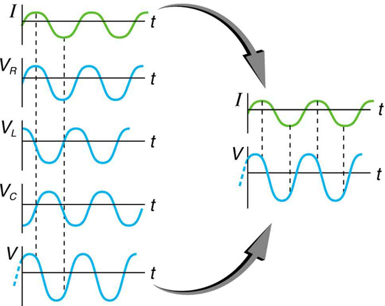
This graph shows the relationships of the voltages in an RLC circuit to the current. The voltages across the circuit elements add to equal the voltage of the source, which is seen to be out of phase with the current.

Calculating impedance and current

An RLC series circuit has a 40.0 Ω resistor, a 3.00 mH inductor, and a 5.00 μF capacitor. (a) Find the circuit’s impedance at 60.0 Hz and 10.0 kHz, noting that these frequencies and the values for L and C are the same as in [link] and [link] . (b) If the voltage source has V rms = 120 V size 12{V rSub { size 8{"rms"} } ="120"`V} {} , what is I rms size 12{I rSub { size 8{"rms"} } } {} at each frequency?

Strategy

For each frequency, we use Z = R 2 + ( X L X C ) 2 size 12{Z= sqrt {R rSup { size 8{2} } + \( X rSub { size 8{L} } - X rSub { size 8{C} } \) rSup { size 8{2} } } } {} to find the impedance and then Ohm’s law to find current. We can take advantage of the results of the previous two examples rather than calculate the reactances again.

Solution for (a)

At 60.0 Hz, the values of the reactances were found in [link] to be X L = 1 . 13 Ω size 12{X rSub { size 8{L} } =1 "." "13" %OMEGA } {} and in [link] to be X C = 531 Ω size 12{X rSub { size 8{C} } ="531 " %OMEGA } {} . Entering these and the given 40.0 Ω for resistance into Z = R 2 + ( X L X C ) 2 size 12{Z= sqrt {R rSup { size 8{2} } + \( X rSub { size 8{L} } - X rSub { size 8{C} } \) rSup { size 8{2} } } } {} yields

Z = R 2 + ( X L X C ) 2 = ( 40 . 0 Ω ) 2 + ( 1 . 13 Ω 531 Ω ) 2 = 531 Ω  at 60 . 0 Hz . alignl { stack { size 12{Z= sqrt {R rSup { size 8{2} } + \( X rSub { size 8{L} } - X rSub { size 8{C} } \) rSup { size 8{2} } } } {} #" "= sqrt { \( "40" "." 0` %OMEGA \) rSup { size 8{2} } + \( 1 "." "13" %OMEGA - "531" %OMEGA \) rSup { size 8{2} } } {} # " "="531" %OMEGA " at 60" "." "0 Hz" {}} } {}

Similarly, at 10.0 kHz, X L = 188 Ω size 12{X rSub { size 8{L} } ="188" %OMEGA } {} and X C = 3 . 18 Ω size 12{X rSub { size 8{C} } =3 "." "18" %OMEGA } {} , so that

Z = ( 40 . 0 Ω ) 2 + ( 188 Ω 3 . 18 Ω ) 2 = 190 Ω  at 10 . 0 kHz. alignl { stack { size 12{Z= sqrt { \( "40" "." 0` %OMEGA \) rSup { size 8{2} } + \( "188" %OMEGA - 3 "." "18" %OMEGA \) rSup { size 8{2} } } } {} #" "="190" %OMEGA " at 10" "." "0 kHz" {} } } {}

Discussion for (a)

In both cases, the result is nearly the same as the largest value, and the impedance is definitely not the sum of the individual values. It is clear that X L size 12{X rSub { size 8{L} } } {} dominates at high frequency and X C size 12{X rSub { size 8{C} } } {} dominates at low frequency.

Solution for (b)

The current I rms size 12{I rSub { size 8{"rms"} } } {} can be found using the AC version of Ohm’s law in Equation I rms = V rms / Z size 12{I rSub { size 8{"rms"} } =V rSub { size 8{"rms"} } /Z} {} :

I rms = V rms Z = 120 V 531 Ω = 0 . 226 A size 12{I rSub { size 8{"rms"} } = { {V rSub { size 8{"rms"} } } over {Z} } = { {"120"" V"} over {"531 " %OMEGA } } =0 "." "226"" A"} {} at 60.0 Hz

Finally, at 10.0 kHz, we find

I rms = V rms Z = 120 V 190 Ω = 0 . 633 A size 12{I rSub { size 8{"rms"} } = { {V rSub { size 8{"rms"} } } over {Z} } = { {"120"" V"} over {"190 " %OMEGA } } =0 "." "633"" A"} {} at 10.0 kHz

Discussion for (a)

The current at 60.0 Hz is the same (to three digits) as found for the capacitor alone in [link] . The capacitor dominates at low frequency. The current at 10.0 kHz is only slightly different from that found for the inductor alone in [link] . The inductor dominates at high frequency.

Resonance in RLC Series ac circuits

How does an RLC circuit behave as a function of the frequency of the driving voltage source? Combining Ohm’s law, I rms = V rms / Z size 12{I rSub { size 8{"rms"} } =V rSub { size 8{"rms"} } /Z} {} , and the expression for impedance Z from Z = R 2 + ( X L X C ) 2 size 12{Z= sqrt {R rSup { size 8{2} } + \( X rSub { size 8{L} } - X rSub { size 8{C} } \) rSup { size 8{2} } } } {} gives

I rms = V rms R 2 + ( X L X C ) 2 . size 12{I rSub { size 8{"rms"} } = { {V rSub { size 8{"rms"} } } over { sqrt {R rSup { size 8{2} } + \( X rSub { size 8{L} } - X rSub { size 8{C} } \) rSup { size 8{2} } } } } } {}

The reactances vary with frequency, with X L size 12{X rSub { size 8{L} } } {} large at high frequencies and X C size 12{X rSub { size 8{C} } } {} large at low frequencies, as we have seen in three previous examples. At some intermediate frequency f 0 size 12{f rSub { size 8{0} } } {} , the reactances will be equal and cancel, giving Z = R size 12{Z=R} {} —this is a minimum value for impedance, and a maximum value for I rms size 12{I rSub { size 8{"rms"} } } {} results. We can get an expression for f 0 size 12{f rSub { size 8{0} } } {} by taking

X L = X C . size 12{X rSub { size 8{L} } =X rSub { size 8{C} } } {}

Substituting the definitions of X L size 12{X rSub { size 8{L} } } {} and X C size 12{X rSub { size 8{C} } } {} ,

2 πf 0 L = 1 2 πf 0 C . size 12{2πf rSub { size 8{0} } L= { {1} over {2πf rSub { size 8{0} } C} } } {}

Solving this expression for f 0 size 12{f rSub { size 8{0} } } {} yields

f 0 = 1 LC , size 12{f rSub { size 8{0} } = { {1} over {2π sqrt { ital "LC"} } } } {}

where f 0 size 12{f rSub { size 8{0} } } {} is the resonant frequency    of an RLC series circuit. This is also the natural frequency at which the circuit would oscillate if not driven by the voltage source. At f 0 size 12{f rSub { size 8{0} } } {} , the effects of the inductor and capacitor cancel, so that Z = R size 12{Z=R} {} , and I rms size 12{I rSub { size 8{"rms"} } } {} is a maximum.

Questions & Answers

differentiate between demand and supply giving examples
Lambiv Reply
differentiated between demand and supply using examples
Lambiv
what is labour ?
Lambiv
how will I do?
Venny Reply
how is the graph works?I don't fully understand
Rezat Reply
information
Eliyee
devaluation
Eliyee
t
WARKISA
hi guys good evening to all
Lambiv
multiple choice question
Aster Reply
appreciation
Eliyee
explain perfect market
Lindiwe Reply
In economics, a perfect market refers to a theoretical construct where all participants have perfect information, goods are homogenous, there are no barriers to entry or exit, and prices are determined solely by supply and demand. It's an idealized model used for analysis,
Ezea
What is ceteris paribus?
Shukri Reply
other things being equal
AI-Robot
When MP₁ becomes negative, TP start to decline. Extuples Suppose that the short-run production function of certain cut-flower firm is given by: Q=4KL-0.6K2 - 0.112 • Where is quantity of cut flower produced, I is labour input and K is fixed capital input (K-5). Determine the average product of lab
Kelo
Extuples Suppose that the short-run production function of certain cut-flower firm is given by: Q=4KL-0.6K2 - 0.112 • Where is quantity of cut flower produced, I is labour input and K is fixed capital input (K-5). Determine the average product of labour (APL) and marginal product of labour (MPL)
Kelo
yes,thank you
Shukri
Can I ask you other question?
Shukri
what is monopoly mean?
Habtamu Reply
What is different between quantity demand and demand?
Shukri Reply
Quantity demanded refers to the specific amount of a good or service that consumers are willing and able to purchase at a give price and within a specific time period. Demand, on the other hand, is a broader concept that encompasses the entire relationship between price and quantity demanded
Ezea
ok
Shukri
how do you save a country economic situation when it's falling apart
Lilia Reply
what is the difference between economic growth and development
Fiker Reply
Economic growth as an increase in the production and consumption of goods and services within an economy.but Economic development as a broader concept that encompasses not only economic growth but also social & human well being.
Shukri
production function means
Jabir
What do you think is more important to focus on when considering inequality ?
Abdisa Reply
any question about economics?
Awais Reply
sir...I just want to ask one question... Define the term contract curve? if you are free please help me to find this answer 🙏
Asui
it is a curve that we get after connecting the pareto optimal combinations of two consumers after their mutually beneficial trade offs
Awais
thank you so much 👍 sir
Asui
In economics, the contract curve refers to the set of points in an Edgeworth box diagram where both parties involved in a trade cannot be made better off without making one of them worse off. It represents the Pareto efficient allocations of goods between two individuals or entities, where neither p
Cornelius
In economics, the contract curve refers to the set of points in an Edgeworth box diagram where both parties involved in a trade cannot be made better off without making one of them worse off. It represents the Pareto efficient allocations of goods between two individuals or entities,
Cornelius
Suppose a consumer consuming two commodities X and Y has The following utility function u=X0.4 Y0.6. If the price of the X and Y are 2 and 3 respectively and income Constraint is birr 50. A,Calculate quantities of x and y which maximize utility. B,Calculate value of Lagrange multiplier. C,Calculate quantities of X and Y consumed with a given price. D,alculate optimum level of output .
Feyisa Reply
Answer
Feyisa
c
Jabir
the market for lemon has 10 potential consumers, each having an individual demand curve p=101-10Qi, where p is price in dollar's per cup and Qi is the number of cups demanded per week by the i th consumer.Find the market demand curve using algebra. Draw an individual demand curve and the market dema
Gsbwnw Reply
suppose the production function is given by ( L, K)=L¼K¾.assuming capital is fixed find APL and MPL. consider the following short run production function:Q=6L²-0.4L³ a) find the value of L that maximizes output b)find the value of L that maximizes marginal product
Abdureman
types of unemployment
Yomi Reply
What is the difference between perfect competition and monopolistic competition?
Mohammed
Got questions? Join the online conversation and get instant answers!
Jobilize.com Reply
Practice Key Terms 4

Get Jobilize Job Search Mobile App in your pocket Now!

Get it on Google Play Download on the App Store Now


Source:  OpenStax, College physics ii. OpenStax CNX. Nov 29, 2012 Download for free at http://legacy.cnx.org/content/col11458/1.2
Google Play and the Google Play logo are trademarks of Google Inc.

Notification Switch

Would you like to follow the 'College physics ii' conversation and receive update notifications?

Ask