6.1 Vector graphics: two-dimensional image representation

Point Matrix. To represent a straight-line image in computer memory, we must store a list of all the endpoints of the line segments that comprise the image. If the point $P_i=(x_i,y_i)$ is such an endpoint, we write it as the column vector

Suppose there are $n$ such endpoints in the entire image. Each point is included only once, even if several lines end at the same point. We can arrange thevectors $P_i$ into a point matrix:

We then store the point matrix $G\in R^{2xn}$ as a two-dimensional array in computer memory.

Consider the list of points

The corresponding point matrix is

Line Matrix. The next thing we need to know is which pairs of points to connect with lines. To store this information for $m$ lines, we will use a line matrix, $H\in R^{2\times m}$ . The line matrix does not store line locations directly. Rather, it contains references to the points stored in $G$ . To indicate a line between points $p_i$ and $p_j$ , we store the indices $i$ and $j$ as a pair. For the $k^{th}$ line in the image, we have the pair

The order of $i$ and $j$ does not really matter since a line from $p_i$ to $p_j$ is the same as a line from $p_j$ to $p_i$ . Next we collect all the lines $h_k$ into a line matrix $H$ :

All the numbers in the line matrix $H$ will be positive integers since they point to columns of $G$ . To find the actual endpoints of a line, we look at columns $i$ and $j$ of the point matrix $G$ .

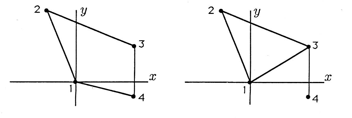
To specify line segments connecting the four points of Example 1 into a quadrilateral, we use the line matrix

Alternatively, we can specify line segments to form a triangle from the first three points plus a line from $P_3$ to $P_4$ :

Figure 1 shows the points $G$ connected first by $H_1$ and then by $H_2.$

Demo 1 (MATLAB) . Use your editor to enter the following MATLAB function file. Save it as vgraphl.m.

After you have saved the function file, run MATLAB and type the following to enter the point and line matrices. (We begin with the transposesof the matrices to make them easier to enter.)

At this point you should use MATLAB's “save” command to save these matrices to a disk file. Type

After you have saved the matrices, use the functionto draw the image by typing VGRAPH1

The advantage of storing points and lines separately is that an object can be moved and scaled by operating only on the point matrix $G$ . The line information in $H$ remains the same since the same pairs of points are connected no matter where we put the points themselves.

Surfaces and Objects. To describe a surface in three dimensions is a fairly complex task, especially if the surface is curved. For this reason, we willbe satisfied with points and lines, sometimes visualizing flat surfaces based on the lines. On the other hand, it is a fairly simple matter to group the pointsand lines into distinct objects . We can define an object matrix K with one column for each object giving the ranges of points and lines associated withthat object. Each column is defined as

As with the line matrix $H$ , the elements of $K$ are integers.

Consider again Demo 1 . We could group the points in $G$ and the lines in $H$ into two objects with the matrix

The first column of $K$ specifies that the first object (Ursa Minor) is made up of points 1 through 7 and lines 1 through 6, and the second column of $K$ defines the second object (Ursa Major) as points 8 through 14 and lines 7 through 12.