

| << Chapter < Page | Chapter >> Page > |
The example in this section addresses sampling, quantization, aliasing and signal reconstruction concepts. [link] shows the completed block diagram of this example, where the following four control parameters are linked to a LabVIEW MathScript node:
Amplitude – to control the amplitude of an input sine wave
Phase – to control the phase of the input signal
Frequency – to control the frequency of the input signal
Sampling frequency – to control the sampling rate of the corresponding discrete signal
Number of quantization levels – to control the number of quantization levels of the corresponding digital signal
To simulate the analog signal via a .m file, consider a very small value of time increment dt (dt = 0.001). To create a discrete signal, sample the analog signal at a rate controlled by the sampling frequency. To simulate the analog signal, use the textual statement
xa=sin(2*pi*f*t) , where t is a vector with increment dt = 0.001. To simulate the discrete signal, use the textual statement
xd=sin(2*pi*f*n) , where n is a vector with increment dn. The ratio dn/dt indicates the number of samples skipped during the sampling process. Again, the ratio of analog frequency to sampling frequency is known as digital or normalized frequency. To convert the discrete signal into a digital one, perform quantization using the LabVIEW MathScript function
round . Set the number of quantization levels as a control.
To reconstruct the analog signal from the digital one, use a linear interpolation technique via the LabVIEW MathScript function
interp
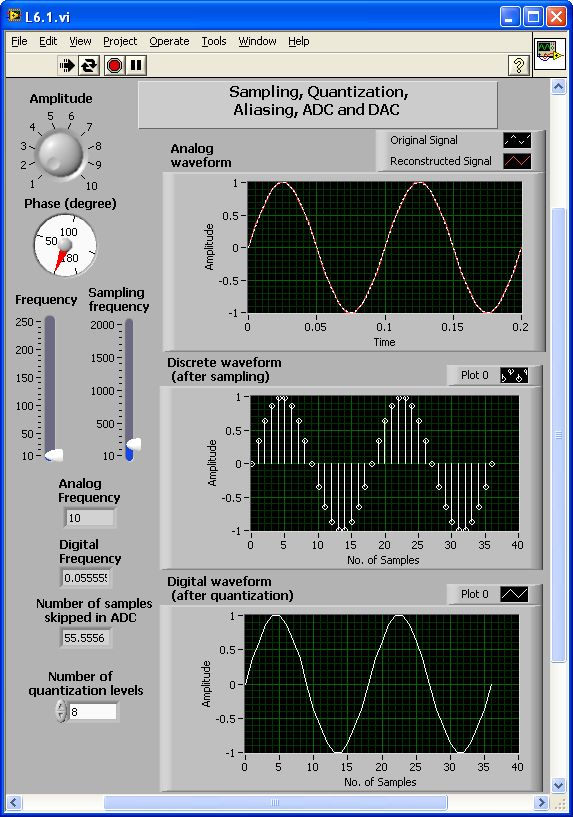
1 . The samples skipped during the sampling process can be recovered after the interpolation. Finally, display the Original signal and the Reconstructed signal in the same graph using the functions Build Waveform, Merge Signal and Waveform Graph. Discrete waveform, Digital waveform, Analog frequency, Digital frequency and Number of samples skipped in ADC are also included in the front panel, shown in
[link] . Use this VI to examine proper signal sampling and reconstruction.

Digital frequency ( ) is related to analog frequency ( ) via the sampling frequency, that is, . Therefore, one can choose the sampling frequency ( ) to increase the digital or normalized frequency of an analog signal by lowering the number of samples.
Set the sampling frequency to Hz and change the analog frequency of the signal. Observe the output for Hz and Hz (See [link] and [link] ). The analog signals appear entirely different in these two cases but the discrete signals are similar. For the second case, the sampling frequency is less than twice that of the analog signal frequency. This violates the Nyquist sampling rate leading to aliasing, which means one does not know from which analog signal the digital signal is created. Note the value of digital frequency is 0.1 radians for the first case and 2.1 radians for the second case. To prevent any aliasing, keep the digital frequency less than 0.5 radians.
Notification Switch
Would you like to follow the 'An interactive approach to signals and systems laboratory' conversation and receive update notifications?

|
|

|
|

|
|
|
|
|

|
|

|
|

|
|

|
|

|
|

|