4.5 Quadratic concepts -- graphing quadratic equations

The graph of the simplest quadratic function, $y=x^2$ , looks like this:

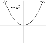
(You can confirm this by plotting points.) The point at the bottom of the U-shaped curve is known as the “vertex.”

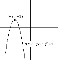
Now consider the function $y=-3{\left(x+2\right)}^2+1$ . It’s an intimidating function, but we have all the tools we need to graph it, based on the permutations we learned in the first unit. Let’s step through them one by one.

• What does the $–$ sign do? It multiplies all $y$ -values by $-1$ ; positive values become negative, and vice-versa. So we are going to get an upside-down U-shape. We say that $y=x^2$ “opens up” and $y=-x^2$ “opens down.”
• What does the 3 do? It multiplies all $y$ -values by 3; positive values become more positive, and negative values become more negative. So it vertical stretches the function.
• What does the $+1$ at the end do? It adds 1 to all $y$ -values, so it moves the function up by 1.
• Finally, what does the $+2$ do? This is a horizontal modification: if we plug in $x=\text{10}$ , we will be evaluating the function at $x=\text{12}$ . In general, we will always be copying the original $x^2$ function to our right ; so we will be 2 units to the left of it.

So what does the graph look like? It has moved 2 to the left and 1 up, so the vertex moves from the origin $(\mathrm{0,0})$ to the point $(-\mathrm{2,1})$ . The graph has also flipped upside-down, and stretched out vertically.

So graphing quadratic functions is easy, no matter how complex they are, if you understand permutations—and if the functions are written in the form $y=a{\left(x-h\right)}^2+k$ , as that one was.

Graphing quadratic functions

But what if the functions are not expressed in that form? We’re more used to seeing them written as $y={\text{ax}}^2+\text{bx}+c$ . For such a function, you graph it by first putting it into the form we used above, and then graphing it. And the way you get it into the right form is...completing the square! This process is almost identical to the way we used completing the square to solve quadratic equations, but some of the details are different.

Graphing a Quadratic Function
Graph ${\mathrm{2x}}^2-\text{20}x+\text{58}$	The problem .
$2\left(x^2-\text{10}x\right)+\text{58}$	We used to start out by dividing both sides by the coefficient of $x^2$ (2 in this case). In this case, we don’t have another side: we can’t make that 2 go away. But it’s still in the way of completing the square. So we factor it out of the first two terms. Do not factor it out of the third (numerical) term; leave that part alone, outside of the parentheses.
$2\left(x^2-\text{10}x+\underline{\text{25}}\right)+\text{58}-\underline{\text{50}}$	Inside the parentheses, add the number you need to complete the square. (Half of 10, squared.)Now, when we add 25 inside the parentheses, what we have really done to our function? We have added 50, since everything in parentheses is doubled. So we keep the function the same by subtracting that 50 right back again, outside the parentheses! Since all we have done in this step is add 50 and then subtract it, the function is unchanged.
$2{\left(x-5\right)}^2+8$	Inside the parentheses, you now have a perfect square and can rewrite it as such. Outside the parentheses, you just have two numbers to combine.
Vertex $\left(\mathrm{5,8}\right)$ opens up	Since the function is now in the correct form, we can read this information straight from the formula and graph it. Note that the number inside the parentheses (the $h$ ) always changes sign; the number outside (the $k$ ) does not.
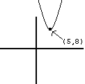	So there’s the graph! It’s easy to draw once you have the vertex and direction. It’s also worth knowing that the 2 vertically stretches the graph, so it will be thinner than a normal $x^2$ .

This process may look intimidating at first. For the moment, don’t worry about mastering the whole thing—instead, look over every individual step carefully and make sure you understand why it works—that is, why it keeps the function fundamentally unchanged, while moving us toward our goal of a form that we can graph.

The good news is, this process is basically the same every time. A different example is worked through in the worksheet “Graphing Quadratic Functions II”—that example differs only because the $x^2$ term does not have a coefficient, which changes a few of the steps in a minor way. You will have plenty of opportunity to practice this process, which will help you get the “big picture” if you understand all the individual steps.

And don’t forget that what we’re really creating here is an algebraic generalization!

This is exactly the sort of generalization we discussed in the first unit—the assertion that these two very different functions will always give the same answer for any $x$ -value you plug into them. For this very reason, we can also assert that the two graphs will look the same. So we can graph the first function by graphing the second.