4.4 Transfer functions and frequency response

We saw in [link] that the transfer function of a linear time-invariant system is given by

If we assume that $H\left(s\right)$ is a rational function of $s$ then we can write

where ${\beta }_1,{\beta }_2,...,{\beta }_q$ are the zeros, and ${\alpha }_1,{\alpha }_2,...,{\alpha }_p$ are the poles of $H\left(s\right)$ . The poles and zeros are points in the $s$ -plane where the transfer function is either non-existent (for a pole) or zero (for a zero). These points can be plotted in the $s$ -plane with “ $\times$ " representing the location of a pole and a “ $\circ$ " representing the location of a zero. Since

we have

and

Each of the quantities $j\Omega -{\beta }_k$ have the same magnitude and phase as a vector from the zero ${\beta }_k$ to the $j\Omega$ axis in the complex $s$ -plane. Likewise, the quantities $j\Omega -{\alpha }_k$ have the same magnitude and phase as vectors from the pole ${\alpha }_k$ to the $j\Omega$ axis.

Example 3.1 Consider a first-order lowpass filter with transfer function

Then

The quantity $j\Omega +2$ has the same magnitude and phase as a vector from the pole at $s=-2$ to the $j\Omega$ axis in the complex plane. The magnitude of the frequency response is the inverse of the magnitude of this vector. The length of $j\Omega +2$ increases as $\Omega$ increases thereby making $\left|H,\left(j,\Omega \right)\right|$ decrease as one would expect of a lowpass filter.

Example 3.2 Consider a first-order highpass filter with transfer function

Then

When $\Omega =0$ , $\left|H,\left(j,\Omega \right)\right|=0$ , but as $\Omega$ approaches infinity, the two vectors $j\Omega$ and $j\Omega +2$ have equal lengths, so the magnitude of the frequency response approaches unity.

Example 3.3 Let's now look at the transfer function corresponding to a second-order filter

Or

The pole-zero plot for this transfer function is shown in [link] . The corresponding magnitude and phase of the frequency response are shown in [link] .

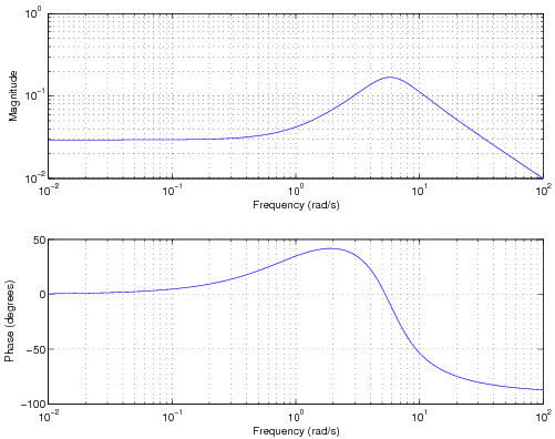
The two poles are at $s=-3\pm j5$ and the zero is at $s=-1$ . When the frequency gets close to either one of the poles, the frequency response magnitude increases since the lengths of one of the vectors $j\Omega \pm j5$ is small.

In the previous example we saw that as the poles get close to the $j\Omega$ axis in the $s$ -plane, the frequency response magnitude increases at frequencies that are close to the poles. In fact, when a pole is located directly on the $j\Omega$ axis, the filter's frequency response magnitude becomes infinite, and will begin to oscillate. If a zero is located on the $j\Omega$ axis, the filters frequency response magnitude will be zero.

Example 3.4 Suppose a filter has transfer function

The two poles are at $s=\pm j5$ and there is a zero at $s=0$ . From [link] , the impulse response of the filter is $h\left(t\right)=cos\left(5t\right)u\left(t\right)$ . This impulse response doesn't die out like most of the impulse responses we've seen. Instead, it oscillates at a fixed frequency. The filter is called an oscillator . Oscillators are useful for generating high-frequency sinusoids used in wireless communications.