Here the "polyphase quadrature" filterbank used in the MPEG audio standards is described in great detail. It has the following practical features: real-valued sub-band outputs, near-perfect reconstruction, and polyphase implementation; and is based on cancellation of adjacent sub-band interference.
Though the uniformly modulated filterbank in
Figure 4 from "Uniformly-Modulated Filterbanks" was shown to have the fast implementation in
Figure 5 from "Uniformly-Modulated Filterbanks" ,
the sub-band outputs are complex-valued for real-valuedinput, hence inconvenient (at first glance
In the structure in
Figure 4 from "Uniformly-Modulated Filterbanks" , it would be reasonable
to replace the standard DFT with a real-valued DFT (defined inthe notes on transform coding), requiring
real-multiplies when
N is a power of 2.
Though it is not clear to the author why such a structure was notadopted in the MPEG standards, the cosine modulated filterbank
derived in this section has equivalent performance and, withits polyphase/DCT implementation, equivalent implementation cost. ) for sub-band coding of real-valued data.
In this section we propose a closely related filterbank with thefollowing properties.
This turns out to be the filterbank specified in the MPEG-1 and 2
(layers 1-3) audio compression standards (see IS0/IEC 13818-3).
Filter design
Real-valued Sub-band Outputs: Recall the generic filterbank structure of
Figure 1 from "Uniformly-Modulated Filterbanks" .
For the sub-band outputs to be real-valued (for real-valued input),we require that the impulse responses of
and
are real-valued.
We can insure this by allocating the
N (symmetric) frequency band pairs
shown in
[link] .
The positive and negative halves of each band pair are centered at
radians.
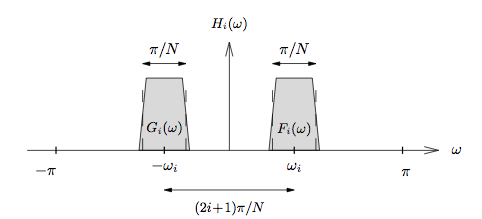
Frequency band pairs for the polyphase quadrature filterbank (
). We can consider each filter
as some combination of
symmetric positive-frequency and negative-frequency components
as shown in
[link] .
Positive- and negative-frequency decomposition of
. Note
will have a similar, if not identical, frequency response. When
and the pairs
are
modulated versions of the same prototype filter
, we can show
that
must be real-valued:
Thus the input to the
reconstruction filter is corrupted by
unwanted spectral images, and the reconstruction filter's job is theremoval of these images.
The reconstruction filter
will have a bandpass frequency response similar (or identical)
to that of
illustrated in
[link] .
Due to the practical design considerations, neither
nor
will be perfect bandpass filters, but we will assume that
the only significant out-of-band energy passed by these filters willoccur in the frequency range just outside of their passbands.
(Note the limited “spillover” in
[link] .)
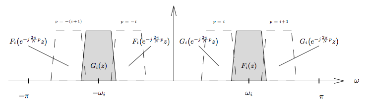
Under these assumptions, the only undesired images in
that will not be completely attenuated by
are the images
adjacent to
and
.
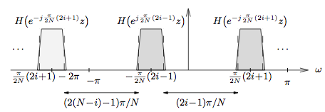
Which indices
p in
[link] (third equation) are responsible for these
adjacent images?
[link] (third equation) implies that index
shifts the frequency
response up by
radians.
Since the passband centers of
and
are
radians apart, the passband of
will reside directly to the left of the passband of
when
.
Similarly, the passband of
will
reside directly to the right of the passband of
when
.
See
[link] for an illustration.
Using the same reasoning, the passband of
will reside directly to the right
of the passband of
when
and directly to the left
when
.
The only exceptions to this rule occur when
, in which case
the images to the right of
and to the left of
are
desired, and when
, in which case the images to the left of
and to the right of
are desired.
Spectral images of
not completely attenuated by
. Based on the arguments above, we can write
, the output of
the
reconstruction filter, as follows:
The previous equation shows that
is corrupted by the portions
of the undesired images not completely removed by the reconstructionfilter
.
In the filterbank context, this undesired behavior is referred to asaliasing.
But notice that aliasing contributions to the signal
will vanish if the inner aliasing components in
cancel the
outer aliasing components in
.
This happens when
which occurs under satisfaction of the two conditions below.
We assume from this point on that the real-valued
filters
and
are constructed using modulated
versions of a lowpass prototype filter
.
(This assumption is required for the existence of a polyphasefilterbank implementation.)
Lets take a closer look at the products
in the previous equation.
As illustrated in
[link] , these products equal
zero when
since their passbands do not overlap.
Setting these products to zero in
[link] (bottom equation) yields the condition
which can also be shown to satisfy
[link] (bottom equation).
Illustration of vanishing terms in
[link] (lower equation). Next we concern ourselves with the requirements on
a
0 and
c
0 .
Assuming
[link] is satisfied, we know that inner aliasing
in
cancels outer aliasing in
for
.
Hence, from
[link] (fourth equation) and
[link] (lower equation),
Noting that the passbands of
and
do not overlap for
, we have
The first two terms in
[link] (third equation) represent aliasing components that
prevent flat overall response at
and
, respectively.
These aliasing terms vanish when
What remains is
Phase Distortion: Perfect reconstruction requires that the analysis/synthesis system hasno phase distortion.
To guarantee the absence of phase distortion, we require that thecomposite system
has a linear phase response.
(Recall that a linear phase response is equivalent to a pure delayin the time domain.)
This linear-phase constraint will provide the final condition used tospecify the constants
and
.
We start by examining the impulse response of
.
Using a technique analogous to
[link] (fifth equation), we can write
Above, we have used the property that multiplication in the
z -domain
implies convolution in the time domain.For
to be linear phase, it's impulse response must be symmetric.
Let us assume that the prototype filter
is linear phase, so that
is symmetric.
Thus
is symmetric about
,
and thus for linear phase
, we require that the quantity
is symmetric about
, i.e.,
for
.
Using trigonometric identities, it can be shown that the condition aboveis equivalent to
which is satisfied when
Restricting
, the previous equation requires that
It can be easily verified that the following
and
satisfy conditions
[link] ,
[link] , and
[link] :
Plugging these into the expression for
we find that
Repeating this procedure for
yields
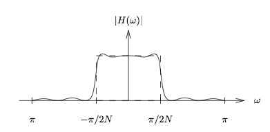
At this point we make a few comments on the design of the lowpass
prototype
.
The perfect
would be an ideal linear-phase lowpass filter with
cutoff at
, as illustrated in
[link] .
Such a filter would perfectly separate the subbands as well as yieldflat composite magnitude response, as per
[link] .
Unfortunately, however, this perfect filter is not realizable with afinite number of filter coefficients.
So, what we really want is a finite-length FIR filter having goodfrequency selectivity, nearly-flat composite response, and linear phase.
The length-512 prototype filter specified in the MPEG standards issuch a filter, as evidenced by the responses in
[link] .
Unfortunately, the standards do not describe how this filter was designed,and a thorough discussion of multirate filter design is outside the
scope of this course. For more on prototype filter design, we point the interested reader to page 358 of Vaidyanathan or Crochiere&Rabiner.
Ideal (dashed) and typical (solid) prototype-filter magnitude responses for the cosine-modulated filterbank. Note bandwidth relative to
[link] .Magnitude response of
of MPEG prototype filter and the resulting composite response
, where
and
. To conclude,
[link] (fourth equation) and
[link] give impulse response expressions
for a set of real-valued filters that comprise a near-perfectlyreconstructing filterbank (under suitable selection of
).
This is commonly referred to
The MPEG standards refer to this filterbank as a “polyphase
quadrature” filterbank (PQF), the name given to the technique byan early technical paper: Rothweiler ICASSP 83 as a “cosine-modulated filterbank” because
all filters are based on cosine modulations of areal-valued linear-phase lowpass prototype
.
The near-perfect reconstruction property follows from the frequency-domaincancellation of adjacent-spectrum aliasing and the lack of phase distortion.
It should be noted that our derivation of the cosine modulated filterbank
is similar to that in Rothweiler ICASSP 83 except for the treatmentsof phase distortion.
See Chapter 8 of Vaidyanathan for a more comprehensiveview of cosine-modulated filterbanks.
Polyphase Implementations: Recall the uniformly modulated filterbank in
Figure 4 from "Uniformly-Modulated Filterbanks" , whose combined modulator-filter coefficients
can be constructed using products of the terms
and
.
Figure 5 from "Uniformly-Modulated Filterbanks" shows a computationally-efficient polyphase/DFT
implementation of the analysis filter which requires only
M multiplies
and one
N -dimensional DFT computation for calculation of
N subband
outputs.We might wonder: Is there a similar polyphase/fast-transform
implementation of the cosine-modulated filterbank derived inthis section?
From
[link] (fourth equation), we see that the impulse responses of
are products of the terms
and
for
.
Note that the inverse-DCT matrix
C
nt can be specified via
components with form similar to the cosine term in
[link] (fourth equation):
Thus it may not be surprising that there exist polyphase/DCT
implementations of the cosine-modulated filterbank.Indeed, one such implementation is specified in the MPEG-2 audio
compression standard (see ISO/IEC 13818-3).This particular implementation is the focus of the next section.
Mpeg filterbank implementation
Since MPEG audio compression standards are so well-known and widespread,
a detailed look at the MPEG filterbank implementation is warranted.The cosine-modulated, or polyphase-quadrature filterbank described
in the previous section is used in MPEG Layers 1-3.(The MPEG hierarchy will be described in a later chapter.)
This section discusses the specific implementation suggested by theMPEG-2 standard (see ISO/IEC 13818-3).
The MPEG standard specifies 512 prototype filter coefficients, the
first of which is zero.To adapt the MPEG filter to our cosine-modulated-filterbank framework,
we append a zero-valued 513
th coefficient so that the resulting
MPEG prototype filter becomes symmetric and hence linear phase.Since the standard specifies
frequency bands, we have
Plugging this value of
M into the filter expressions
[link] (fourth equation) and
[link] , the
-periodicity of the cosine
implies that they may be rewritten as follows.
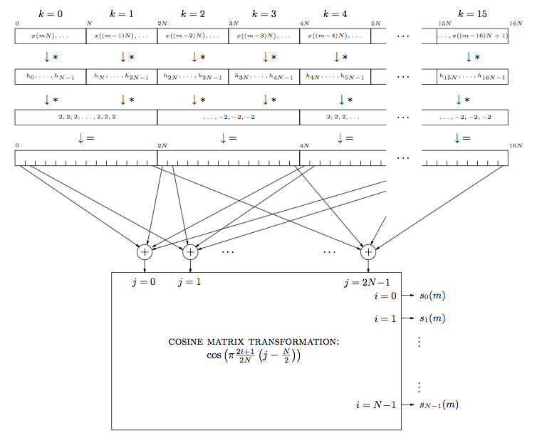
Encoding: Here we derive the encoder filterbank implementation suggested in theMPEG-2 standard (see ISO/IEC 13818-3).
Using
to denote the output of the
analysis filter,
we have
The relationship between
and its downsampled version
is given by
so that the downsampled analysis output
can be written as
Using the substitution
for
,
[link] illustrates this process.
MPEG encoder filterbank implementation suggested in ISO/IEC 13818-3.
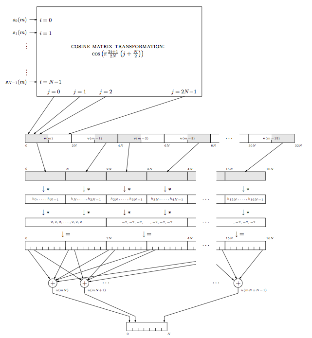
Decoding: Here we derive the dencoder filterbank implementation suggested in theMPEG-2 standard (see ISO/IEC 13818-3).
Using
to denote the output of the
upsampler,
The input to the upsampler
is related to the output
by
so that
Lets write
for
and
for
.
Then due to the restricted ranges of
ℓ and
q ,
Using these substitutions in the previous equation for
,
Summing
over
i to create
,
If we define
(note the range of
!) then we can rewrite
[link] illustrates the construction of
using the notation
MPEG decoder filterbank implementation suggested in ISO/IEC 13818-3.
DCT Implementation of Cosine Matrixing: As seen in
[link] and
[link] ,
the filterbank implementations suggested by the MPEG standard requirea cosine matrix operation that, if implemented using straightforward
arithmetic, requires
multiply/adds at both
the encoder and decoder.Note, however, that the cosine transformations in
[link] and
[link] do bear a great deal of similarity to the DCT:
which we know has a fast algorithm:
Lee's
fast-DCT, for example, requires only 80
multiplications and 209 additions (see B.G.Lee TASSP Dec 84).So how do we implement the matrix operation using the fast-DCT?
A technique has been described clearly in Konstantinides SPL 1994,the results of which are summarized below.
At the encoder, the matrix operation can be written
where
is created from
by windowing, shifting, and adding.
(See
[link] .)
We can write
where, for
,
is the following manipulation
of
:
Compare
[link] to the inverse DCT in
[link] (lower equation).
At the decoder, the matrix operation can be written
where
are windowed, shifted,
and added to compute
.
(See
[link] .) It is shown in Konstantinides SPL 1994 that,
for
,
can be calculated by first computing
:
and rearranging the outputs according to
Compare
[link] to the DCT in
[link] (upper equation).
Receive real-time job alerts and never miss the right job again
Source:
OpenStax, An introduction to source-coding: quantization, dpcm, transform coding, and sub-band coding. OpenStax CNX. Sep 25, 2009 Download for free at http://cnx.org/content/col11121/1.2
Google Play and the Google Play logo are trademarks of Google Inc.
Notification Switch
Would you like to follow the 'An introduction to source-coding: quantization, dpcm, transform coding, and sub-band coding' conversation and receive update notifications?


![This figure is a cartesian graph, with horizontal axis ω, and an unlabeled vertical axis. The graph consists of eight colored, connected rectangles of identical dimension, beginning. The rectangles all have one side drawn on the base of the graph. The leftmost rectangle's left side is located at a ω-value of -π, and the rightmost rectangles right side is located at a ω-value of π. The midpoint along the horizontal axis of each rectangle is labeled from left to right as -ω_3, -ω_2, -ω_1, -ω_0, ω_0, ω_1, ω_2, and ω_3. The rectangles from left to right are colored green, red, blue, grey, grey, blue, red, green. Above the left side of the graph is a horizontal arrow pointing in both directions, labeled π/N. Above the right side of the graph is the equation ω_i = [(2i + 1)π]/2N.](/ocw/mirror/col11121_1.2_complete/m32148/img033.png)
![This figure is a cartesian graph, with horizontal axis ω, and an unlabeled vertical axis. The graph consists of eight colored, connected rectangles of identical dimension, beginning. The rectangles all have one side drawn on the base of the graph. The leftmost rectangle's left side is located at a ω-value of -π, and the rightmost rectangles right side is located at a ω-value of π. The midpoint along the horizontal axis of each rectangle is labeled from left to right as -ω_3, -ω_2, -ω_1, -ω_0, ω_0, ω_1, ω_2, and ω_3. The rectangles from left to right are colored green, red, blue, grey, grey, blue, red, green. Above the left side of the graph is a horizontal arrow pointing in both directions, labeled π/N. Above the right side of the graph is the equation ω_i = [(2i + 1)π]/2N.](img033.eps)


![This figure is comprised of two cartesian graphs. Both graphs show waves plotted with radians on the horizontal axis and magnitude [dB] on the vertical axis. The first graph is titled prototype filter. The vertical values on this graph range from -120 to 20, and the horizontal values from 0 to 3. The graph begins at nearly a vertical value of 20, immediately falling into a series of nonuniform waves of varying amplitudes and wavelengths in no distinct pattern. There are perhaps one hundred of these waves, never reaching a vertical value again higher than -80, and continuing to the right side of the graph. The second graph is titled composite system. The vertical values range from -2 x 10^-4 to 8 x 10^-4. The horizontal values range from 0 to 3. The waves in this graph follow a rigid, predictable pattern. They have extremely short wavelengths and there are perhaps 150 waves occurring across the page. The waves are centered around a vertical value of 3, and follow a repeating amplitude pattern of 3.2, 3.1, 3.1, 3.2, 2.5.](/ocw/mirror/col11121_1.2_complete/m32148/img038.png)
![This figure is comprised of two cartesian graphs. Both graphs show waves plotted with radians on the horizontal axis and magnitude [dB] on the vertical axis. The first graph is titled prototype filter. The vertical values on this graph range from -120 to 20, and the horizontal values from 0 to 3. The graph begins at nearly a vertical value of 20, immediately falling into a series of nonuniform waves of varying amplitudes and wavelengths in no distinct pattern. There are perhaps one hundred of these waves, never reaching a vertical value again higher than -80, and continuing to the right side of the graph. The second graph is titled composite system. The vertical values range from -2 x 10^-4 to 8 x 10^-4. The horizontal values range from 0 to 3. The waves in this graph follow a rigid, predictable pattern. They have extremely short wavelengths and there are perhaps 150 waves occurring across the page. The waves are centered around a vertical value of 3, and follow a repeating amplitude pattern of 3.2, 3.1, 3.1, 3.2, 2.5.](img038.eps)