

| << Chapter < Page | Chapter >> Page > |
If you strain your eyes and you know exactly where to look, you may be able to see a single black spike with an amplitude of 180 at the far left of the topplot. If you can't see it, you will simply have to trust me when I tell you that it is there.
Now take a look at the amplitude spectrum in the second plot from the top. What you should see is a straight black line extending from zero to the foldingfrequency on the right. This is because such an impulse (theoretically) contains an equal distribution of energy at every frequency from zero toinfinity.
(In reality, there is no such thing as a perfect impulse, so there is no such thing as infinite bandwidth. However, the bandwidth of a practicalimpulse is very wide and the amplitude spectrum is very flat.)
That is one of the things that make the impulse so useful. It is often used for various testing purposes in both the analog world and the digital world.
Now look at the real spectrum in the second plot from the top. As you can see, it looks exactly like the amplitude spectrum. This is because the impulseappears at zero time. We will change this in the next experiment so that you can see the impact of a time delay on the complex spectrum.
Moving on down the page, the imaginary part of the spectrum is a flat line with a value of zero across the entire frequency range. Once again, this isbecause the impulse appears at zero time.
Because the imaginary value is zero everywhere, the ratio of the imaginary value to the real value is also zero everywhere. Thus, the phase angle is alsozero at all frequencies within the range.
Now we are going to introduce a one-sample time delay in the location of the impulse relative to the time origin. We will keep the zero time reference at thefirst sample and cause the impulse to appear as the second sample in the eleven-sample sequence.
The new parameters are shown in Figure 6 . The only change is the move of the impulse from the first sample in the eleven-sample pulse to the second sample inthe eleven-sample pulse.
| Figure 6. Introduce a time delay. |
|---|
Parameters read from file
Data length: 400Pulse length: 11
Sample for zero time: 0Lower frequency bound: 0.0
Upper frequency bound: 0.5Pulse Values
0.0180.0
0.00.0
0.00.0
0.00.0
0.00.0
0.0 |
The result of performing the spectral analysis on this new time series is shown in Figure 7 .
| Figure 7. Spectral analysis of an impulse with a one-sample delay. |
|---|
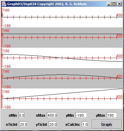 |
Once again, if you strain your eyes, you may be able to see the impulse on the left end of the top plot. It has been shifted one sample to the rightrelative to that shown in Figure 5 .
The amplitude spectrum in the second plot looks exactly like it looked in Figure 5 . That is as it should be. The spectral content of a pulse is determined by its waveform, not by its location in time. Simply moving the impulse by onesample into the future doesn't change its spectral content.
Notification Switch
Would you like to follow the 'Digital signal processing - dsp' conversation and receive update notifications?

|
|

|
|

|
|

|
|

|
|

|
|

|
|

|
|

|
|

|