4.2 Direction fields and numerical methods

For the rest of this chapter we will focus on various methods for solving differential equations and analyzing the behavior of the solutions. In some cases it is possible to predict properties of a solution to a differential equation without knowing the actual solution. We will also study numerical methods for solving differential equations, which can be programmed by using various computer languages or even by using a spreadsheet program, such as Microsoft Excel.

Creating direction fields

Direction fields (also called slope fields) are useful for investigating first-order differential equations. In particular, we consider a first-order differential equation of the form

An applied example of this type of differential equation appears in Newton’s law of cooling, which we will solve explicitly later in this chapter. First, though, let us create a direction field for the differential equation

Here $T\left(t\right)$ represents the temperature (in degrees Fahrenheit) of an object at time $t,$ and the ambient temperature is $72\text{°}\text{F}\text{.}$ [link] shows the direction field for this equation.

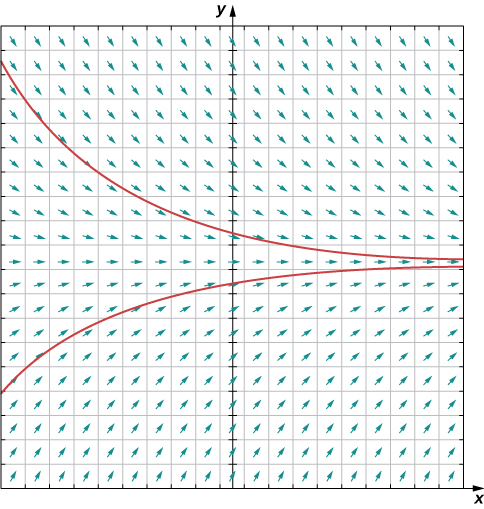
The idea behind a direction field is the fact that the derivative of a function evaluated at a given point is the slope of the tangent line to the graph of that function at the same point. Other examples of differential equations for which we can create a direction field include

To create a direction field, we start with the first equation: $y\prime =3x+2y-4.$ We let $\left(x_0,y_0\right)$ be any ordered pair, and we substitute these numbers into the right-hand side of the differential equation. For example, if we choose $x=1\text{and}y=2,$ substituting into the right-hand side of the differential equation yields

This tells us that if a solution to the differential equation $y\prime =3x+2y-4$ passes through the point $\left(1,2\right),$ then the slope of the solution at that point must equal $3.$ To start creating the direction field, we put a short line segment at the point $\left(1,2\right)$ having slope $3.$ We can do this for any point in the domain of the function $f\left(x,y\right)=3x+2y-4,$ which consists of all ordered pairs $\left(x,y\right)$ in ${ℝ}^2.$ Therefore any point in the Cartesian plane has a slope associated with it, assuming that a solution to the differential equation passes through that point. The direction field for the differential equation $y^{\prime }=3x+2y-4$ is shown in [link] .

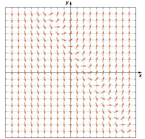
We can generate a direction field of this type for any differential equation of the form $y\prime =f\left(x,y\right).$