3.6 The functions e^x and e^jθ: numerical experiment (approximating

We have demonstrated that the function $e^{j\theta }$ has two representations:

1. $e^{j\theta }=\underset{n\to \infty }{lim}{(1+\frac{j\theta }{n})}^n$ ; and
2. $e^{j\theta }=\underset{n\to \infty }{lim}\sum k=0n\frac{{\left(j\theta \right)}^k}{k!}$ .

In this experiment, you will write a MATLAB program to evaluate the two functions $f_n$ and $S_n$ for twenty values of $n$ :

1. $f_n={(1+\frac{j\theta }{n})}^n,n=1,2,...,20$ ; and
2. $S_n=\sum k=0n\frac{(j\theta {)}^k}{k!},n=1,2,...,20k$ .

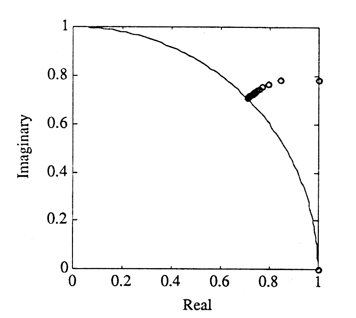
Choose $\theta =\pi /4(=pi/4)$ . Use an implicitloop to draw and plot a circle of radius 1. Then use an implicit for loop to compute and plot $f_n$ and an explicit for loop to compute and plot $S_n$ for $n=1,2,...,100$ . You should observe plots like those illustrated in [link] . Interpret them. for