<< Chapter < Page Chapter >> Page >
This figure has two graphs, both of the same non-negative function in the first quadrant. The function increases and decreases. The quadrant is divided into a grid. The first graph, beginning on the x-axis at the point labeled x sub 0, there are trapezoids shaded whose heights are represented by the function p(x), which is a curve following an approximate path of the original graph. The x-axis is scaled by increments of x sub 0, x sub 1, x sub 2. The second graph has on the x-axis at the point labeled x sub 0. There are shaded regions under the curve, divided by x sub 0, x sub 1, x sub 2, x sub 3, and x sub 4. The curve is sectioned into two different parts above the shaded areas. These two parts are labeled p sub 1(x) and p sub 2(x).
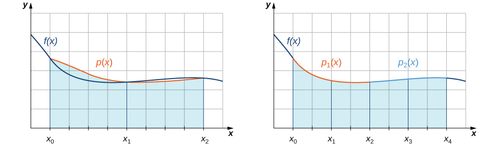
With Simpson’s rule, we approximate a definite integral by integrating a piecewise quadratic function.

To understand the formula that we obtain for Simpson’s rule, we begin by deriving a formula for this approximation over the first two subintervals. As we go through the derivation, we need to keep in mind the following relationships:

f ( x 0 ) = p ( x 0 ) = A x 0 2 + B x 0 + C f ( x 1 ) = p ( x 1 ) = A x 1 2 + B x 1 + C f ( x 2 ) = p ( x 2 ) = A x 2 2 + B x 2 + C

x 2 x 0 = 2 Δ x , where Δ x is the length of a subinterval.

x 2 + x 0 = 2 x 1 , since x 1 = ( x 2 + x 0 ) 2 .

Thus,

x 0 x 2 f ( x ) d x x 0 x 2 p ( x ) d x = x 0 x 2 ( A x 2 + B x + C ) d x = A 3 x 3 + B 2 x 2 + C x | x 2 x 0 Find the antiderivative. = A 3 ( x 2 3 x 0 3 ) + B 2 ( x 2 2 x 0 2 ) + C ( x 2 x 0 ) Evaluate the antiderivative. = A 3 ( x 2 x 0 ) ( x 2 2 + x 2 x 0 + x 0 2 ) + B 2 ( x 2 x 0 ) ( x 2 + x 0 ) + C ( x 2 x 0 ) = x 2 x 0 6 ( 2 A ( x 2 2 + x 2 x 0 + x 0 2 ) + 3 B ( x 2 + x 0 ) + 6 C ) Factor out x 2 x 0 6 . = Δ x 3 ( ( A x 2 2 + B x 2 + C ) + ( A x 0 2 + B x 0 + C ) + A ( x 2 2 + 2 x 2 x 0 + x 0 2 ) + 2 B ( x 2 + x 0 ) + 4 C ) = Δ x 3 ( f ( x 2 ) + f ( x 0 ) + A ( x 2 + x 0 ) 2 + 2 B ( x 2 + x 0 ) + 4 C ) Rearrange the terms. Factor and substitute. f ( x 2 ) = A x 0 2 + B x 0 + C and f ( x 0 ) = A x 0 2 + B x 0 + C . = Δ x 3 ( f ( x 2 ) + f ( x 0 ) + A ( 2 x 1 ) 2 + 2 B ( 2 x 1 ) + 4 C ) Substitute x 2 + x 0 = 2 x 1 . = Δ x 3 ( f ( x 2 ) + 4 f ( x 1 ) + f ( x 0 ) ) . Expand and substitute f ( x 1 ) = A x 1 2 + B x 1 + .

If we approximate x 2 x 4 f ( x ) d x using the same method, we see that we have

x 0 x 4 f ( x ) d x Δ x 3 ( f ( x 4 ) + 4 f ( x 3 ) + f ( x 2 ) ) .

Combining these two approximations, we get

x 0 x 4 f ( x ) d x = Δ x 3 ( f ( x 0 ) + 4 f ( x 1 ) + 2 f ( x 2 ) + 4 f ( x 3 ) + f ( x 4 ) ) .

The pattern continues as we add pairs of subintervals to our approximation. The general rule may be stated as follows.

Simpson’s rule

Assume that f ( x ) is continuous over [ a , b ] . Let n be a positive even integer and Δ x = b a n . Let [ a , b ] be divided into n subintervals, each of length Δ x , with endpoints at P = { x 0 , x 1 , x 2 ,… , x n } . Set

S n = Δ x 3 ( f ( x 0 ) + 4 f ( x 1 ) + 2 f ( x 2 ) + 4 f ( x 3 ) + 2 f ( x 4 ) + + 2 f ( x n 2 ) + 4 f ( x n 1 ) + f ( x n ) ) .

Then,

lim n + S n = a b f ( x ) d x .

Just as the trapezoidal rule is the average of the left-hand and right-hand rules for estimating definite integrals, Simpson’s rule may be obtained from the midpoint and trapezoidal rules by using a weighted average. It can be shown that S 2 n = ( 2 3 ) M n + ( 1 3 ) T n .

It is also possible to put a bound on the error when using Simpson’s rule to approximate a definite integral. The bound in the error is given by the following rule:

Rule: error bound for simpson’s rule

Let f ( x ) be a continuous function over [ a , b ] having a fourth derivative, f ( 4 ) ( x ) , over this interval. If M is the maximum value of | f ( 4 ) ( x ) | over [ a , b ] , then the upper bound for the error in using S n to estimate a b f ( x ) d x is given by

Error in S n M ( b a ) 5 180 n 4 .

Applying simpson’s rule 1

Use S 2 to approximate 0 1 x 3 d x . Estimate a bound for the error in S 2 .

Since [ 0 , 1 ] is divided into two intervals, each subinterval has length Δ x = 1 0 2 = 1 2 . The endpoints of these subintervals are { 0 , 1 2 , 1 } . If we set f ( x ) = x 3 , then

S 4 = 1 3 · 1 2 ( f ( 0 ) + 4 f ( 1 2 ) + f ( 1 ) ) = 1 6 ( 0 + 4 · 1 8 + 1 ) = 1 4 . Since f ( 4 ) ( x ) = 0 and consequently M = 0 , we see that

Error in S 2 0 ( 1 ) 5 180 2 4 = 0 .

This bound indicates that the value obtained through Simpson’s rule is exact. A quick check will verify that, in fact, 0 1 x 3 d x = 1 4 .

Got questions? Get instant answers now!

Applying simpson’s rule 2

Use S 6 to estimate the length of the curve y = 1 2 x 2 over [ 1 , 4 ] .

The length of y = 1 2 x 2 over [ 1 , 4 ] is 1 4 1 + x 2 d x . If we divide [ 1 , 4 ] into six subintervals, then each subinterval has length Δ x = 4 1 6 = 1 2 , and the endpoints of the subintervals are { 1 , 3 2 , 2 , 5 2 , 3 , 7 2 , 4 } . Setting f ( x ) = 1 + x 2 ,

S 6 = 1 3 · 1 2 ( f ( 1 ) + 4 f ( 3 2 ) + 2 f ( 2 ) + 4 f ( 5 2 ) + 2 f ( 3 ) + 4 f ( 7 2 ) + f ( 4 ) ) .

After substituting, we have

S 6 = 1 6 ( 1.4142 + 4 · 1.80278 + 2 · 2.23607 + 4 · 2.69258 + 2 · 3.16228 + 4 · 3.64005 + 4.12311 ) 8.14594.
Got questions? Get instant answers now!
Practice Key Terms 5

Get Jobilize Job Search Mobile App in your pocket Now!

Get it on Google Play Download on the App Store Now


Source:  OpenStax, Calculus volume 2. OpenStax CNX. Feb 05, 2016 Download for free at http://cnx.org/content/col11965/1.2
Google Play and the Google Play logo are trademarks of Google Inc.

Notification Switch

Would you like to follow the 'Calculus volume 2' conversation and receive update notifications?

Ask