<< Chapter < Page Chapter >> Page >

Use the midpoint rule with n = 2 to estimate 1 2 1 x d x .

24 35

Got questions? Get instant answers now!

The trapezoidal rule

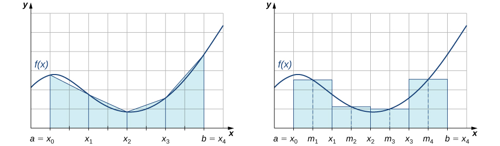
We can also approximate the value of a definite integral by using trapezoids rather than rectangles. In [link] , the area beneath the curve is approximated by trapezoids rather than by rectangles.

This figure is a graph of a non-negative function in the first quadrant. The function increases and decreases. The quadrant is divided into a grid. Beginning on the x-axis at the point labeled a = x sub 0, there are trapezoids shaded whose heights are approximately the height of the curve. The x-axis is scaled by increments of a = x sub 0, x sub 1, x sub 2, x sub 3, and b = x sub 4.
Trapezoids may be used to approximate the area under a curve, hence approximating the definite integral.

The trapezoidal rule for estimating definite integrals uses trapezoids rather than rectangles to approximate the area under a curve. To gain insight into the final form of the rule, consider the trapezoids shown in [link] . We assume that the length of each subinterval is given by Δ x . First, recall that the area of a trapezoid with a height of h and bases of length b 1 and b 2 is given by Area = 1 2 h ( b 1 + b 2 ) . We see that the first trapezoid has a height Δ x and parallel bases of length f ( x 0 ) and f ( x 1 ) . Thus, the area of the first trapezoid in [link] is

1 2 Δ x ( f ( x 0 ) + f ( x 1 ) ) .

The areas of the remaining three trapezoids are

1 2 Δ x ( f ( x 1 ) + f ( x 2 ) ) , 1 2 Δ x ( f ( x 2 ) + f ( x 3 ) ) , and 1 2 Δ x ( f ( x 3 ) + f ( x 4 ) ) .

Consequently,

a b f ( x ) d x 1 2 Δ x ( f ( x 0 ) + f ( x 1 ) ) + 1 2 Δ x ( f ( x 1 ) + f ( x 2 ) ) + 1 2 Δ x ( f ( x 2 ) + f ( x 3 ) ) + 1 2 Δ x ( f ( x 3 ) + f ( x 4 ) ) .

After taking out a common factor of 1 2 Δ x and combining like terms, we have

a b f ( x ) d x 1 2 Δ x ( f ( x 0 ) + 2 f ( x 1 ) + 2 f ( x 2 ) + 2 f ( x 3 ) + f ( x 4 ) ) .

Generalizing, we formally state the following rule.

The trapezoidal rule

Assume that f ( x ) is continuous over [ a , b ] . Let n be a positive integer and Δ x = b a n . Let [ a , b ] be divided into n subintervals, each of length Δ x , with endpoints at P = { x 0 , x 1 , x 2 , x n } . Set

T n = 1 2 Δ x ( f ( x 0 ) + 2 f ( x 1 ) + 2 f ( x 2 ) + + 2 f ( x n 1 ) + f ( x n ) ) .

Then, lim n + T n = a b f ( x ) d x .

Before continuing, let’s make a few observations about the trapezoidal rule. First of all, it is useful to note that

T n = 1 2 ( L n + R n ) where L n = i = 1 n f ( x i 1 ) Δ x and R n = i = 1 n f ( x i ) Δ x .

That is, L n and R n approximate the integral using the left-hand and right-hand endpoints of each subinterval, respectively. In addition, a careful examination of [link] leads us to make the following observations about using the trapezoidal rules and midpoint rules to estimate the definite integral of a nonnegative function. The trapezoidal rule tends to overestimate the value of a definite integral systematically over intervals where the function is concave up and to underestimate the value of a definite integral systematically over intervals where the function is concave down. On the other hand, the midpoint rule tends to average out these errors somewhat by partially overestimating and partially underestimating the value of the definite integral over these same types of intervals. This leads us to hypothesize that, in general, the midpoint rule tends to be more accurate than the trapezoidal rule.

This figure has two graphs, both of the same non-negative function in the first quadrant. The function increases and decreases. The quadrant is divided into a grid. The first graph, beginning on the x-axis at the point labeled a = x sub 0, there are trapezoids shaded whose heights are approximately the height of the curve. The x-axis is scaled by increments of a = x sub 0, xsub1, x sub 2, x sub 3, and b = x sub 4. The second graph has on the x-axis at the point labeled a = x sub 0. There are rectangles shaded whose heights are approximately the height of the curve. The x-axis is scaled by increments of m sub 1, x sub 1, m sub 2, x sub 2, m sub 3, x sub 3, m sub 4 and b = x sub 4.
The trapezoidal rule tends to be less accurate than the midpoint rule.

Using the trapezoidal rule

Use the trapezoidal rule to estimate 0 1 x 2 d x using four subintervals.

The endpoints of the subintervals consist of elements of the set P = { 0 , 1 4 , 1 2 , 3 4 , 1 } and Δ x = 1 0 4 = 1 4 . Thus,

0 1 x 2 d x 1 2 · 1 4 ( f ( 0 ) + 2 f ( 1 4 ) + 2 f ( 1 2 ) + 2 f ( 3 4 ) + f ( 1 ) ) = 1 8 ( 0 + 2 · 1 16 + 2 · 1 4 + 2 · 9 16 + 1 ) = 11 32 .
Got questions? Get instant answers now!

Use the trapezoidal rule with n = 2 to estimate 1 2 1 x d x .

17 24

Got questions? Get instant answers now!

Absolute and relative error

An important aspect of using these numerical approximation rules consists of calculating the error in using them for estimating the value of a definite integral. We first need to define absolute error    and relative error    .

Practice Key Terms 5

Get Jobilize Job Search Mobile App in your pocket Now!

Get it on Google Play Download on the App Store Now


Source:  OpenStax, Calculus volume 2. OpenStax CNX. Feb 05, 2016 Download for free at http://cnx.org/content/col11965/1.2
Google Play and the Google Play logo are trademarks of Google Inc.

Notification Switch

Would you like to follow the 'Calculus volume 2' conversation and receive update notifications?

Ask