3.4 Elliptic-function filter properties  (Page 3/5)

which, on removing the parameter $n$ , become

or

These relationships are central to the design of elliptic- function filters. $N$ is an odd integer which is the order of the filter. For $N=5$ , the resulting rational function is shown in [link] .

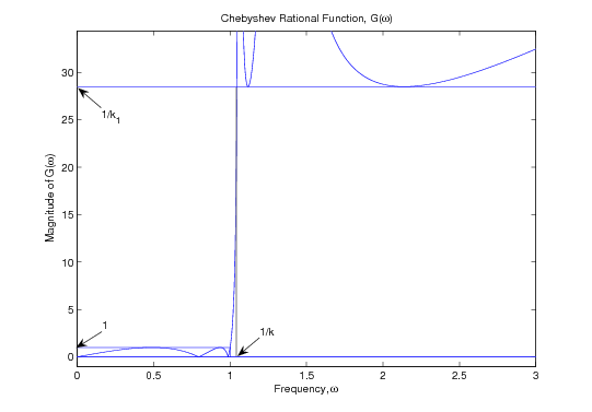
This function is the basis of the approximation necessary for the optimal filter frequency response. It approximates zero over thefrequency range $-1<\omega <1$ by an equal-ripple oscillation between $\pm 1$ . It also approximates infinity over the range $1/k<\left|\omega \right|<\infty$ by a reciprocal oscillation that keeps $\left|F\left(\omega \right)\right|>1/k_1$ . The zero approximation is normalized in both the frequency range and the $F\left(\omega \right)$ values to unity. The infinity approximation has its frequency range set by the choice of the modulus $k$ , and the minimum value of $\left|F\right(\omega \left)\right|$ is set by the choice of the second modulus $k_1$ .

If $k$ and $k_1$ are determined from the filter specifications, they in turn determine the complementary moduli $k^{\text{'}}$ and $k_1^{\text{'}}$ , which altogether determine the four values of the complete ellipticintegral $K$ needed to determine the order $N$ in [link] . In general, this sequence of events will not result in an integer. Inpractice, however, the next larger integer is used, and either $k$ or $k_1$ (or perhaps both) is altered to satisfy [link] .

In addition to the two-band equal-ripple characteristics, $G\left(\omega \right)$ has another interesting and valuable property. The pole and zero locations have a reciprocal relationship that can be expressedby

where

This states that if the zeros of $G\left(\omega \right)$ are located at ${\omega }_{zi}$ , the poles are located at

If the zeros are known, the poles are known, and vice versa. A similar relation exists between the points of zero derivatives inthe 0 to 1 region and those in the $1/k$ to infinity region.

The zeros of $G\left(\omega \right)$ are found from [link] by requiring

which implies

From [link] , this gives

This can be reformulated using [link] so that $n$ and $K_1$ are not needed. For $N$ odd, the zero locations are

The pole locations are found from these zero locations using [link] . The locations of the zero-derivative points are given by

in the 0 to 1 region, and the corresponding points inthe 1/k to infinity region are found from [link] .

The above relations assume N to be an odd integer. A modification for N even is necessary. For proper alignment of thereal periods, the original definition of $G\left(\omega \right)$ is changed to

which gives for the zero locations with N even

The even and odd N cases can be combined to give

for

with the poles determined from [link] .

Note that it is possible to determine $G\left(\omega \right)$ from k and N without explicitly using $k_1$ or $n$ . Values for $k_1$ and $n$ are implied by the requirements of [link] or [link] .

Zero locations

The locations of the zeros of the filter transfer function $F\left(\omega \right)$ are easily found since they are the same as the poles of $G\left(\omega \right)$ , given in [link] .

for