

| << Chapter < Page | Chapter >> Page > |
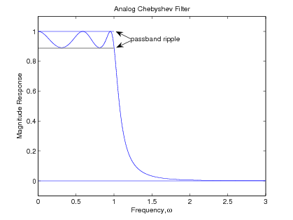
The approximation parameters must be clearly understood. The passband ripple is defined to be the difference between the maximumand the minumum of over the passband frequencies of . There can be confusion over this point as two definitions appear in the literature. Most digital [link] , [link] , [link] , [link] and analog [link] filter design books use the definition just stated. Approximation literature, especiallyconcerning FIR filters, use one half this value which is a measure of the maximum error, , where is the center line in the passband of [link] , which oscillates around.
The Chebyshev theory states that the maximum error over that band is minimum and that this optimal approximation function hasequal ripple over the pass band. It is easy to see that e in [link] determines the ripple in the passband and the order determines the rate that the response goes to zero as goes to infinity.
A method for finding the pole locations for the Chebyshev filter transfer function is next developed. The details of thissection can be skipped and the results in [link] , [link] used if desired.
From [link] , it is seen that the poles of occur when
or
From [link] , define with real and imaginary parts given by
This gives,
which implies the real part of is zero. This requires
which implies
which in turn implies that takes on values of
For these values of , , we have
which requires to take on a value of
Using gives
which gives the location of the poles in the plane as
where
for values of where
A partially factored form for F(s) can be derived using the same approach as for the Butterworth filter. For N even, the form is
for . For odd, has a single real pole and, therefore, the form
for This is a convenient form for the cascade and parallel realizations.
A single formula for both even and odd N is
for values of where
Note the similarity to the pole locations for the Butterworth filter. Cross multiplying, squaring, and adding the terms in [link] , [link] gives
This is the equation for an ellipse and shows that the poles of a Chebyshev filter lie on an ellipse similarto the way the poles of a Butterworth filter lie on a circle [link] , [link] , [link] , [link] , [link] , [link] .
This section has developed the classical Chebyshev filter approximation which minimizes the maximum error over the passbandand uses a Taylor's series approximation at infinity. This results in the error being equal ripple in the passband. Thetransfer function was developed in terms of the Chebyshev polynomial and explicit formulas were derived for the location ofthe transfer function poles. These can be expressed as a modification of the pole locations for the Butterworth filter andare implemented in the appendix.
Notification Switch
Would you like to follow the 'Digital signal processing and digital filter design (draft)' conversation and receive update notifications?

|
|

|
|

|
|

|
|

|
|

|
|

|
|

|
|

|
|

|