3.1 The functions e^x and e^jθ: the function e^x

Many of you know the number e as the base of the natural logarithm, which has the value 2.718281828459045. . . . What you may not know is thatthis number is actually defined as the limit of a sequence of approximating numbers. That is,

This means, simply, that the sequence of numbers ${(1+1)}^1,{(1+\frac{1}{2})}^2,{(1+\frac{1}{3})}^3$ , . . . , gets arbitrarily close to 2.718281828459045. . . . But why should sucha sequence of numbers be so important? In the next several paragraphs we answer this question.

Derivatives and the Number $e$ . The number $f_n={(1+\frac{1}{n})}^n$ arises in the study of derivatives in the following way. Consider the function

and ask yourself when the derivative of $f\left(x\right)$ equals $f\left(x\right)$ . The function $f\left(x\right)$ is plotted in [link] for $a>1$ . The slope of the function at point $x$ is

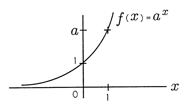
If there is a special value for a such that

then $\frac{d}{dx}f\left(x\right)$ would equal $f\left(x\right)$ . We call this value of $a$ the special (or exceptional) number $e$ and write

The number $e$ would then be $e=f\left(1\right)$ . Let's write our condition that $\frac{a^{\Delta x}-1}{\Delta x}$ converges to 1 as

or as

Our definition of $e=\underset{n\to \infty }{lim}{(1+\frac{1}{n})}^{1/n}$ amounts to defining $\Delta x=\frac{1}{n}$ and allowing $n\to \infty$ in order to make $\Delta x\to 0$ . With this definition for $e$ , it is clear that the function $e^x$ is defined to be ${\left(e\right)}^x$ :

By letting $\Delta x=\frac{x}{n}$ we can write this definition in the more familiar form

This is our fundamental definition for the function $e^x$ . When evaluated at $x=1$ , it produces the definition of $e$ given in [link] .

The derivative of $e^x$ is, of course,

This means that Taylor's theoremmay be used to find another characterization for $e^x$ : Taylor's theorem says that a function may be completely characterized by all of its derivatives (provided they all exist).

When this series expansion for $e^x$ is evaluated at $x=1$ , it produces the following series for $e$ :

In this formula, $n$ ! is the product $n(n-1)(n-2)\cdots \left(2\right)1$ . Read $n$ ! as " $n$ factorial.”

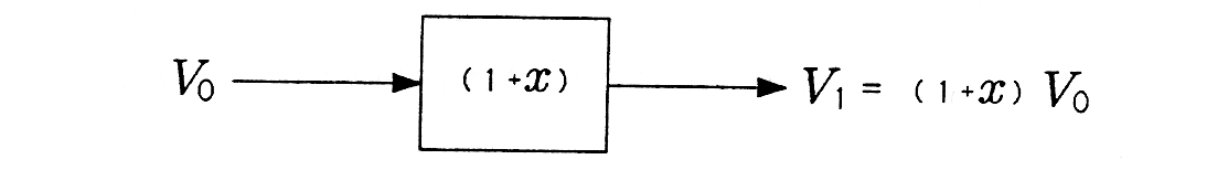
Compound Interest and the Function $e^x$ . There is an example from your everyday life that shows even more dramatically how the function $e^x$ arises. Suppose you invest $V_0$ dollars in a savings account that offers $100x$ % annual interest. (When $x=0.01$ , this is 1%; when $x=0.10$ , this is 10% interest.) If interest is compounded only once per year, you have the simple interest formula for $V_1$ , the value of your savings account after 1 compound (in this case, 1 year):

$V_1=(1+x)V_0$ . This result is illustrated in the block diagram of Figure 2.2(a). In this diagram,your input fortune V ₀ is processed by the “interest block” to produce your output fortune V ₁ . If interest is compounded monthly, then the annual interest is divided into 12 equal parts and applied 12 times. The compounding formulafor V ₁₂ , the value of your savings after 12 compounds (also 1 year) is

This result is illustrated in [link] . Can you read the block diagram? The general formula for the value of an account that is compounded n times per year is

$V_n$ is the value of your account after $n$ compounds in a year, when the annual interest rate is 100x%.

Bankers have discovered the (apparent) appeal of infinite, or continuous, compounding:

We know that this is just

So, when deciding between $100x_1$ % interest compounded daily and $100x_2\%$ interest compounded continuously, we need only compare

We suggest that daily compounding is about as good as continuous compounding. What do you think? How about monthly compounding?