

| << Chapter < Page | Chapter >> Page > |
1. Load the data in Stata from Excel .
2. Convert MSAT and VSAT to MSAT/100 and VSAT/100, respectively, using the commands:
.replace msat = msat/100
.replace vsat = vsat/100
3. Common sense dictates that we should calculate the means and standard deviations of the variables to be sure that there are no entry errors. We need to construct a table that compares the means and standard deviations reported in BFS with those in our dataset. Table 2, which has the means and standard deviations reported by BFS, gives a place to put the means and standard deviations for the variables in our dataset. Fill in the information missing from Table 2.
| Our data | Butler, et al. | |||
| Variable | Mean | Std. Dev. | Mean | Std. Dev. |
| msat | 6.25 | 0.60 | ||
| foreign | 0.11 | 0.32 | ||
| female | 0.39 | 0.49 | ||
| emecon | 0.34 | 0.48 | ||
| emoss | 0.17 | 0.38 | ||
| emns | 0.21 | 0.41 | ||
| emh | 0.07 | 0.25 | ||
| am1 | 0.49 | 0.50 | ||
| am2 | 0.45 | 0.50 | ||
| am3 | 0.01 | 0.11 | ||
| phy1 | 0.67 | 0.47 | ||
| Phy2 | 0.02 | 0.14 | ||
| chem1 | 0.82 | 0.39 | ||
| chem2 | 0.12 | 0.32 |
4. Estimate the ordered probit regression using (in Stata ) the commands:
.global indvar msat foreign female emecon emoss emns emh am1 am2 am3 phy1 phy2 chem1 chem2
.oprobit highestmath $indvar
5. Use the result of this estimation to complete Table 3. One way to make the conversion from the Stata output to the neater table relatively easily is to follow these steps: (1) replace each double space by a single space until there were none left; (2) replace each space with a tab (^t); (3) convert the material into a table using the "Insert/Table" command with a tab as the separator; and (4) clean up the table by moving the data into an Excel file, fixing the formatting, and returning the data to the Word file (alternatively, you can use formatting commands in Stata to control how the output appears).
| highestmath | Coef. | Std. Err. | z | P>z | [95% Conf. Interval] | |
| msat1 | ||||||
| foreign | ||||||
| female | ||||||
| emecon | ||||||
| emoss | ||||||
| emns | ||||||
| emh | ||||||
| am1 | ||||||
| am2 | ||||||
| am3 | ||||||
| phy1 | ||||||
| Phy2 | ||||||
| chem1 | ||||||
| chem2 | ||||||
| _cut1 | ||||||
| _cut2 | ||||||
| _cut3 | ||||||
| _cut4 | ||||||
| _cut5 | ||||||
| _cut6 | ||||||
| Observations | ||||||
| Log likelihood | ||||||
| LR χ 2 (14) | ||||||
| Prob>χ 2 | ||||||
| Pueudo-R 2 |
6. Compare your results with the table reported in the article. The table in the article is Table II on page 193 and is reproduced in Figure 3. What we are interested in is comparing column 4 in Figure 3 with columns 2 and 4 in Table 3. Table 4 below offers a model for this comparison.
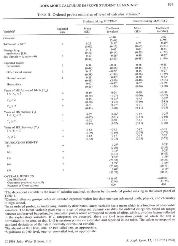
Table 4. Comparison of ordered probit estimations.
| Our estimates | Butler, et al. estimates | |||
| Estimate | z | Estimate | t-value | |
| msat1 | 0.05 | 6.12 | ||
| foreign | 0.02 | 0.14 | ||
| female | 0.25 | 2.59 | ||
| emecon | -0.11 | 0.86 | ||
| emoss | -0.29 | 1.99 | ||
| emns | 0.43 | 3.10 | ||
| emh | -0.37 | 1.78 | ||
| am1 | 0.24 | 1.07 | ||
| am2 | 0.93 | 4.04 | ||
| am3 | 0.77 | 1.70 | ||
| phy1 | 0.26 | 2.71 | ||
| Phy2 | 0.38 | 1.07 | ||
| chem1 | -0.12 | 0.69 | ||
| chem2 | 0.17 | 0.75 | ||
| Intercept | -3.09 | 5.48 | ||
| _cut1 | 0.27 | 7.29 | ||
| _cut2 | 0.33 | 8.16 | ||
| _cut3 | 1.52 | 20.32 | ||
| _cut4 | 1.79 | 23.07 | ||
| _cut5 | 2.04 | 23.72 | ||
| _cut6 |
7. It is easy to see from Table 4 is that almost without exception the estimates of the parameters and their t-ratios are very similar. The exception arises with the estimates of the truncation points (_cut# in the Stata results). We will have to figure out what these are estimates of in order to make sense of them. Figure 1 shows the "cutoffs" that are being estimated. Footnote c in the BFS Table II on page 193 (shown in Figure 3) offers a useful observation:
Notification Switch
Would you like to follow the 'Econometrics for honors students' conversation and receive update notifications?

|
|

|
|

|
|

|
|

|
|

|
|
|
|
|

|
|

|
|

|