

| << Chapter < Page | Chapter >> Page > |
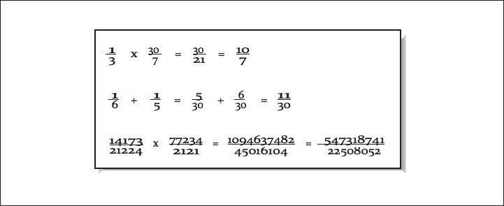
The limitation that occurs when using rational numbers to represent real numbers is that the size of the numerators and denominators tends to grow. For each addition, a common denominator must be found. To keep the numbers from becoming extremely large, during each operation, it is important to find the greatest common divisor (GCD) to reduce fractions to their most compact representation. When the values grow and there are no common divisors, either the large integer values must be stored using dynamic memory or some form of approximation must be used, thus losing the primary advantage of rational numbers.
For mathematical packages such as Maple or Mathematica that need to produce exact results on smaller data sets, the use of rational numbers to represent real numbers is at times a useful technique. The performance and storage cost is less significant than the need to produce exact results in some instances.
If the desired number of decimal places is known in advance, it’s possible to use fixed-point representation. Using this technique, each real number is stored as a scaled integer. This solves the problem that base-10 fractions such as 0.1 or 0.01 cannot be perfectly represented as a base-2 fraction. If you multiply 110.77 by 100 and store it as a scaled integer 11077, you can perfectly represent the base-10 fractional part (0.77). This approach can be used for values such as money, where the number of digits past the decimal point is small and known.
However, just because all numbers can be accurately represented it doesn’t mean there are not errors with this format. When multiplying a fixed-point number by a fraction, you get digits that can’t be represented in a fixed-point format, so some form of rounding must be used. For example, if you have $125.87 in the bank at 4% interest, your interest amount would be $5.0348. However, because your bank balance only has two digits of accuracy, they only give you $5.03, resulting in a balance of $130.90. Of course you probably have heard many stories of programmers getting rich depositing many of the remaining 0.0048 amounts into their own account. My guess is that banks have probably figured that one out by now, and the bank keeps the money for itself. But it does make one wonder if they round or truncate in this type of calculation. Perhaps banks round this instead of truncating, knowing that they will always make it up in teller machine fees.
The floating-point format that is most prevalent in high performance computing is a variation on scientific notation. In scientific notation the real number is represented using a mantissa, base, and exponent: 6.02 × 10 23 .
The mantissa typically has some fixed number of places of accuracy. The mantissa can be represented in base 2, base 16, or BCD. There is generally a limited range of exponents, and the exponent can be expressed as a power of 2, 10, or 16.
The primary advantage of this representation is that it provides a wide overall range of values while using a fixed-length storage representation. The primary limitation of this format is that the difference between two successive values is not uniform. For example, assume that you can represent three base-10 digits, and your exponent can range from –10 to 10. For numbers close to zero, the “distance” between successive numbers is very small. For the number , the next larger number is . The distance between these two “close” small numbers is 0.000000000001. For the number , the next larger number is . The distance between these “close” large numbers is 100 million.
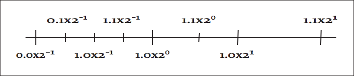
In [link] , we use two base-2 digits with an exponent ranging from –1 to 1.
Distance between successive floating-point numbers
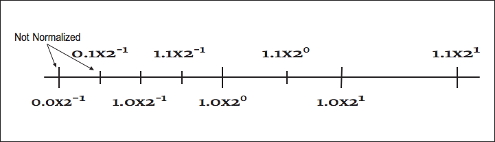
There are multiple equivalent representations of a number when using scientific notation:
By convention, we shift the mantissa (adjust the exponent) until there is exactly one nonzero digit to the left of the decimal point. When a number is expressed this way, it is said to be “normalized.” In the above list, only 6.00 × 10 5 is normalized. [link] shows how some of the floating-point numbers from [link] are not normalized.
While the mantissa/exponent has been the dominant floating-point approach for high performance computing, there were a wide variety of specific formats in use by computer vendors. Historically, each computer vendor had their own particular format for floating-point numbers. Because of this, a program executed on several different brands of computer would generally produce different answers. This invariably led to heated discussions about which system provided the right answer and which system(s) were generating meaningless results. Interestingly, there was an easy answer to the question for many programmers. Generally they trusted the results from the computer they used to debug the code and dismissed the results from other computers as garbage.
When storing floating-point numbers in digital computers, typically the mantissa is normalized, and then the mantissa and exponent are converted to base-2 and packed into a 32- or 64-bit word. If more bits were allocated to the exponent, the overall range of the format would be increased, and the number of digits of accuracy would be decreased. Also the base of the exponent could be base-2 or base-16. Using 16 as the base for the exponent increases the overall range of exponents, but because normalization must occur on four-bit boundaries, the available digits of accuracy are reduced on the average. Later we will see how the IEEE 754 standard for floating-point format represents numbers.
Notification Switch
Would you like to follow the 'Cómputo de alto rendimiento' conversation and receive update notifications?

|
|

|
|

|
|

|
|

|
|

|
|

|
|

|
|

|
|
|
|