<< Chapter < Page Chapter >> Page >

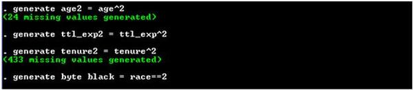
Additionally, because race is a categorical variable that has three potential values—1 if white, 2 if black, and 3 otherwise—we have to create a dummy variable in order to use this variable. The transformations we use are shown in Figure 3.

Stata commands to transform the data.
Transformations of the variables to create new variables.

The last step before estimating the regressions is to identify the data set as a panel data. shows the two commands that must be entered in order for Stata to know that idcode is the individual category and that year is the time series variable. Figure 4 shows these two commands.

Declaring the category and time identifiers.

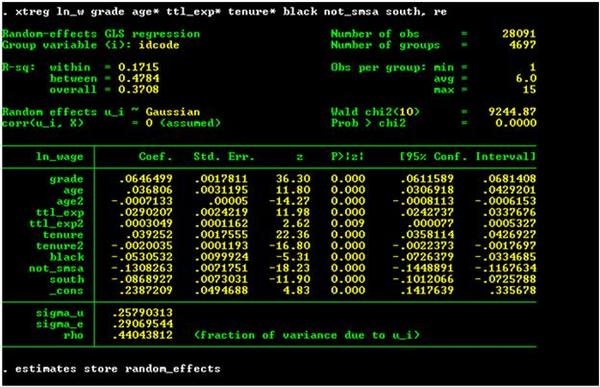
We are now ready to estimate the model (the natural logarithm of wages as a function of various variables). We begin with the random-effects model. Figure 5 shows the command and the results of the estimation of the random-effects model. There are several things to note here. First, in the command we are able to refer to all variables that have age in them by using age* , the * tells Stata to use and variable that begins with the letters age. Second, we will need to use the estimation results in the Hausman test. Thus, we have stored these results in “random_effects” using the command estimates store random_effects .

Stata output from the random-effects estimation.
The random-effects estimation.

Notice that three R-squared values are reported in Figure 5. Also, wages reach a peak when the woman is 0.036806 2 ( 0.0007133 ) = 25.7998 MathType@MTEF@5@5@+=feaagyart1ev2aqatCvAUfeBSjuyZL2yd9gzLbvyNv2CaerbuLwBLnhiov2DGi1BTfMBaeXatLxBI9gBaerbd9wDYLwzYbItLDharqqtubsr4rNCHbGeaGqiVu0Je9sqqrpepC0xbbL8F4rqqrFfpeea0xe9Lq=Jc9vqaqpepm0xbba9pwe9Q8fs0=yqaqpepae9pg0FirpepeKkFr0xfr=xfr=xb9adbaqaaeGaciGaaiaabeqaamaabaabaaGcbaGaeyOeI0YaaSaaaeaacaaIWaGaaiOlaiaaicdacaaIZaGaaGOnaiaaiIdacaaIWaGaaGOnaaqaaiaaikdadaqadaqaaiabgkHiTiaaicdacaGGUaGaaGimaiaaicdacaaIWaGaaG4naiaaigdacaaIZaGaaG4maaGaayjkaiaawMcaaaaacqGH9aqpcaaIYaGaaGynaiaac6cacaaI3aGaaGyoaiaaiMdacaaI4aaaaa@4CCE@ years old and after 9.795857 years on the job. The interpretation of the other variables demands a bit of algebra. For instance, the fact that black is a dummy variable affects our interpretation; when an individual is a black, her wage level is: ln w B = β 0 + β 1 + . MathType@MTEF@5@5@+=feaagyart1ev2aaatCvAUfeBSjuyZL2yd9gzLbvyNv2CaerbuLwBLnhiov2DGi1BTfMBaeXatLxBI9gBaerbd9wDYLwzYbItLDharqqtubsr4rNCHbGeaGqiVu0Je9sqqrpepC0xbbL8F4rqqrFfpeea0xe9Lq=Jc9vqaqpepm0xbba9pwe9Q8fs0=yqaqpepae9pg0FirpepeKkFr0xfr=xfr=xb9adbaqaaeGaciGaaiaabeqaamaabaabaaGcbaGaciiBaiaac6gacaWG3bWaaSbaaSqaaiaadkeaaeqaaOGaeyypa0JaeqOSdi2aaSbaaSqaaiaaicdaaeqaaOGaey4kaSIaeqOSdi2aaSbaaSqaaiaaigdaaeqaaOGaey4kaSIaeS47IWKaaiOlaaaa@445D@ When she is nonblack, her wage level is ln w N B = β 0 + . MathType@MTEF@5@5@+=feaagyart1ev2aaatCvAUfeBSjuyZL2yd9gzLbvyNv2CaerbuLwBLnhiov2DGi1BTfMBaeXatLxBI9gBaerbd9wDYLwzYbItLDharqqtubsr4rNCHbGeaGqiVu0Je9sqqrpepC0xbbL8F4rqqrFfpeea0xe9Lq=Jc9vqaqpepm0xbba9pwe9Q8fs0=yqaqpepae9pg0FirpepeKkFr0xfr=xfr=xb9adbaqaaeGaciGaaiaabeqaamaabaabaaGcbaGaciiBaiaac6gacaWG3bWaaSbaaSqaaiaad6eacaWGcbaabeaakiabg2da9iabek7aInaaBaaaleaacaaIWaaabeaakiabgUcaRiabl+Uimjaac6caaaa@41BC@ Thus, we have: ln w B ln w N B = β 1 MathType@MTEF@5@5@+=feaagyart1ev2aaatCvAUfeBSjuyZL2yd9gzLbvyNv2CaerbuLwBLnhiov2DGi1BTfMBaeXatLxBI9gBaerbd9wDYLwzYbItLDharqqtubsr4rNCHbGeaGqiVu0Je9sqqrpepC0xbbL8F4rqqrFfpeea0xe9Lq=Jc9vqaqpepm0xbba9pwe9Q8fs0=yqaqpepae9pg0FirpepeKkFr0xfr=xfr=xb9adbaqaaeGaciGaaiaabeqaamaabaabaaGcbaGaciiBaiaac6gacaWG3bWaaSbaaSqaaiaadkeaaeqaaOGaeyOeI0IaciiBaiaac6gacaWG3bWaaSbaaSqaaiaad6eacaWGcbaabeaakiabg2da9iabek7aInaaBaaaleaacaaIXaaabeaaaaa@42FB@ or w B w N B = e β 1 = e 0.0530532 = 0.94833. MathType@MTEF@5@5@+=feaagyart1ev2aaatCvAUfeBSjuyZL2yd9gzLbvyNv2CaerbuLwBLnhiov2DGi1BTfMBaeXatLxBI9gBaerbd9wDYLwzYbItLDharqqtubsr4rNCHbGeaGqiVu0Je9sqqrpepC0xbbL8F4rqqrFfpeea0xe9Lq=Jc9vqaqpepm0xbba9pwe9Q8fs0=yqaqpepae9pg0FirpepeKkFr0xfr=xfr=xb9adbaqaaeGaciGaaiaabeqaamaabaabaaGcbaWaaSaaaeaacaWG3bWaaSbaaSqaaiaadkeaaeqaaaGcbaGaam4DamaaBaaaleaacaWGobGaamOqaaqabaaaaOGaeyypa0JaamyzamaaCaaaleqabaGaeqOSdi2aaSbaaWqaaiaaigdaaeqaaaaakiabg2da9iaadwgadaahaaWcbeqaaiabgkHiTiaaicdacaGGUaGaaGimaiaaiwdacaaIZaGaaGimaiaaiwdacaaIZaGaaGOmaaaakiabg2da9iaaicdacaGGUaGaaGyoaiaaisdacaaI4aGaaG4maiaaiodacaGGUaaaaa@5001@ Thus, the wage level of a black is, everything else held constant, 94.8 percent of the wage level of a nonblack.

If we assume that grade is a continuous variable (it really is not), we have the following interpretation of the parameter: ln w = β 0 + β 1 g r a d e + MathType@MTEF@5@5@+=feaagyart1ev2aaatCvAUfeBSjuyZL2yd9gzLbvyNv2CaerbuLwBLnhiov2DGi1BTfMBaeXatLxBI9gBaerbd9wDYLwzYbItLDharqqtubsr4rNCHbGeaGqiVu0Je9sqqrpepC0xbbL8F4rqqrFfpeea0xe9Lq=Jc9vqaqpepm0xbba9pwe9Q8fs0=yqaqpepae9pg0FirpepeKkFr0xfr=xfr=xb9adbaqaaeGaciGaaiaabeqaamaabaabaaGcbaGaciiBaiaac6gacaWG3bGaeyypa0JaeqOSdi2aaSbaaSqaaiaaicdaaeqaaOGaey4kaSIaeqOSdi2aaSbaaSqaaiaaigdaaeqaaOGaam4zaiaadkhacaWGHbGaamizaiaadwgacqGHRaWkcqWIVlctaaa@474A@ implies that 1 w w g r a d e = β 1 MathType@MTEF@5@5@+=feaagyart1ev2aaatCvAUfeBSjuyZL2yd9gzLbvyNv2CaerbuLwBLnhiov2DGi1BTfMBaeXatLxBI9gBaerbd9wDYLwzYbItLDharqqtubsr4rNCHbGeaGqiVu0Je9sqqrpepC0xbbL8F4rqqrFfpeea0xe9Lq=Jc9vqaqpepm0xbba9pwe9Q8fs0=yqaqpepae9pg0FirpepeKkFr0xfr=xfr=xb9adbaqaaeGaciGaaiaabeqaamaabaabaaGcbaWaaSaaaeaacaaIXaaabaGaam4DaaaadaWcaaqaaiabgkGi2kaadEhaaeaacqGHciITcaWGNbGaamOCaiaadggacaWGKbGaamyzaaaacqGH9aqpcqaHYoGydaWgaaWcbaGaaGymaaqabaaaaa@43BC@ . Thus, in our case a increase of 1 year of schooling causes wages to increase by 6.46 percent.

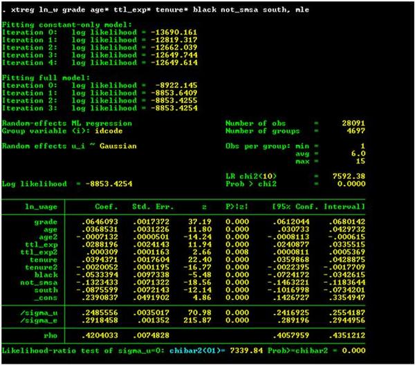
We can compare the results of using the re option with using the mle option (which directs Stata to use maximum likelihood techniques to estimate the parameters of the system. The mle parameter estimates, shown in Figure 6, are the same as those generated using the re command. However, the estimates of the standard errors (and, thus, the z-values) are different.

Stata output from the maximum likelihood estimation.
The maximum likelihood estimation.

The estimation of the fixed-effects model is straightforward and is shown in Figure 7. The command is the same as in the random-effects model but with the re replaced by fe . Notice from the results that the variables grade and black are dropped from the estimation results. They are dropped because the amount of schooling and race of an individual is fixed over all observations. These two variables, thus, are perfectly correlated with the dummy variables that hold constant the individual level characteristics. The effects of education and race differences are absorbed into the residual.

Get Jobilize Job Search Mobile App in your pocket Now!

Get it on Google Play Download on the App Store Now


Source:  OpenStax, Econometrics for honors students. OpenStax CNX. Jul 20, 2010 Download for free at http://cnx.org/content/col11208/1.2
Google Play and the Google Play logo are trademarks of Google Inc.

Notification Switch

Would you like to follow the 'Econometrics for honors students' conversation and receive update notifications?

Ask