

| << Chapter < Page | Chapter >> Page > |
A second downside of this representation is called the curse of dimensionality . Suppose , and we discretize each of the dimensions of the state into values. Then the total number of discrete states we have is . This grows exponentially quickly in the dimension of the state space , and thus does not scale well to large problems. For example, with a 10d state,if we discretize each state variable into 100 values, we would have discrete states, which is far too many to represent even on a modern desktop computer.
As a rule of thumb, discretization usually works extremely well for 1d and 2d problems (and has the advantage of being simple and quick to implement).Perhaps with a little bit of cleverness and some care in choosing the discretization method, it often works well for problems with up to 4d states. Ifyou're extremely clever, and somewhat lucky, you may even get it to work for some 6d problems. But it very rarely works for problems any higherdimensional than that.
We now describe an alternative method for finding policies in continuous-state MDPs, in which we approximate directly, without resorting to discretization. This approach, caled value function approximation, has been successfully applied to many RL problems.
To develop a value function approximation algorithm, we will assume that we have a model , or simulator , for the MDP. Informally, a simulator is a black-box that takes as input any (continuous-valued) state and action , and outputs a next-state sampled according to the state transition probabilities :
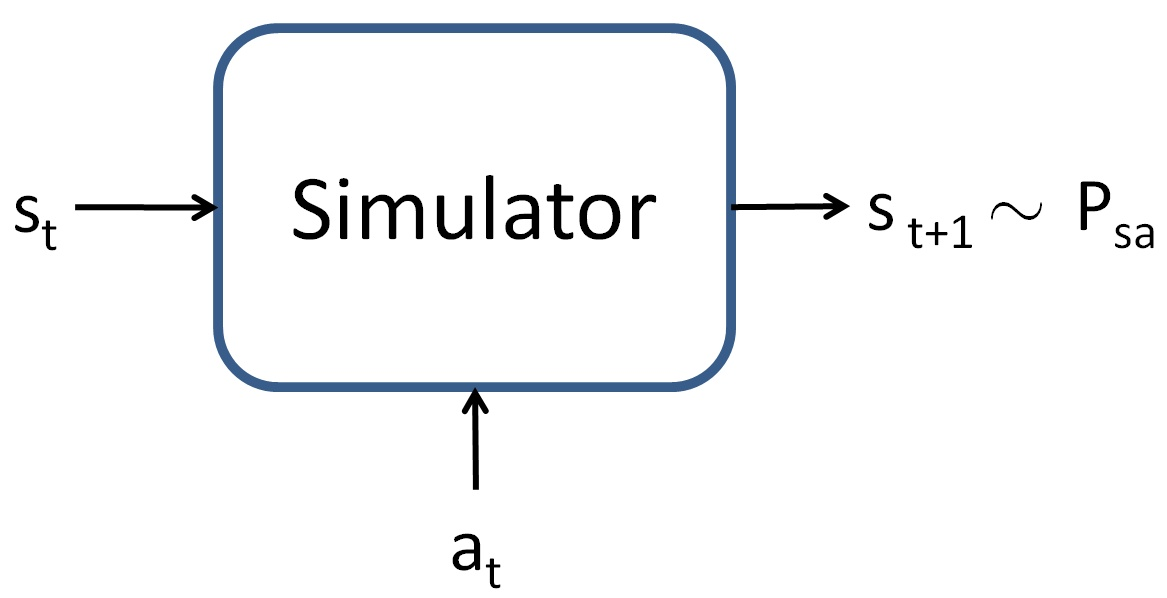
simulation. For example, the simulator for the inverted pendulum in PS4 was obtained by using the laws of physics to calculate what position andorientation the cart/pole will be in at time , given the current state at time and the action taken, assuming that we know all the parameters of the system such as the length of the pole, the mass of the pole, and so on.Alternatively, one can also use an off-the-shelf physics simulation software package which takes as input a complete physical description of a mechanicalsystem, the current state and action , and computes the state of the system a small fraction of a second into the future. Open Dynamics Engine (http://www.ode.com) is one example of a free/open-source physics simulator that can be used to simulate systems like theinverted pendulum, and that has been a reasonably popular choice among RL researchers.
An alternative way to get a model is to learn one from data collected in the MDP. For example, suppose we execute trials in which we repeatedly take actions in an MDP, each trial for timesteps. This can be done picking actions at random, executing some specific policy, or via some other way of choosing actions. We would then observe state sequences like the following:
We can then apply a learning algorithm to predict as a function of and .
Notification Switch
Would you like to follow the 'Machine learning' conversation and receive update notifications?

|
|

|
|

|
|

|
|

|
|

|
|

|
|

|
|

|
|
|
|