

| << Chapter < Page | Chapter >> Page > |
Determine the value of each of the following.
>>(6*7)+4^2-2^4 (ans = 42)
>>((3^2+2^3)/(4^5-5^4))+((sqrt(64)-5^2)/(4^5+5^6+7^8)) (ans = 0.0426)
>>log10(10^2)+10^5 (ans = 100002)
>>exp(2)+2^3-log(exp(2)) (ans = 13.3891)
>>sin(2*pi)+cos(pi/4) (ans = 0.7071)
>>tan(pi/3)+cos(270*pi/180)+sin(270*pi/180)+cos(pi/3) (ans = 1.2321)
Solve the following system of equations:
>>A=[2 4; 1 5]

A =2     4
     1     5>>B=[1; 2]

B =1
     2>>Solution=A\B

Solution =-0.5000
    0.5000
Evaluate y at 5.
>>p=[4 0 3 -1 0]

p =4     0     3    -1     0>>polyval(p,5)

ans =2570>>
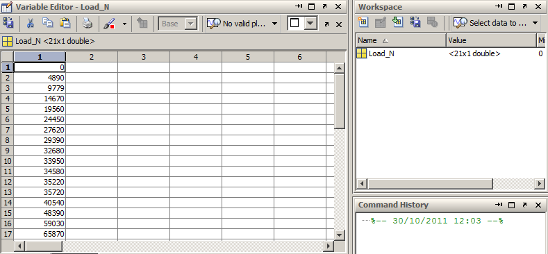
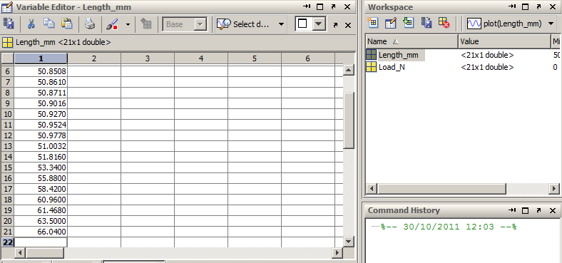
Given below is Load-Gage Length data for a type 304 stainless steel that underwent a tensile test. Original specimen diameter is 12.7 mm. Introduction to Materials Science for Engineers by J. F. Shackelford, Macmillan Publishing Company. © 1985, (p.304)
| Load [N] | Gage Length [mm] |
|---|---|
| 0.000 | 50.8000 |
| 4890 | 50.8102 |
| 9779 | 50.8203 |
| 14670 | 50.8305 |
| 19560 | 50.8406 |
| 24450 | 50.8508 |
| 27620 | 50.8610 |
| 29390 | 50.8711 |
| 32680 | 50.9016 |
| 33950 | 50.9270 |
| 34580 | 50.9524 |
| 35220 | 50.9778 |
| 35720 | 51.0032 |
| 40540 | 51.816 |
| 48390 | 53.340 |
| 59030 | 55.880 |
| 65870 | 58.420 |
| 69420 | 60.960 |
| 69670 (maximum) | 61.468 |
| 68150 | 63.500 |
| 60810 (fracture) | 66.040 (after fracture) |
First, we need to enter the data sets. Because it is rather a large table, using Variable Editor is more convenient. See the figures below:
Next, we will calculate the cross-sectional area.
Area=pi/4*(0.0127^2)

Area =1.2668e-004
Now, we can find the Stress values with the following, note that we are obtaining results in MPa:
Sigma=(Load_N./Area)*10^(-6)

Sigma =0
   38.602277.1964
  115.8065154.4086
  193.0108218.0351
  232.0076257.9792
  268.0047272.9780
  278.0302281.9773
  320.0269381.9955
  465.9888519.9844
  548.0085549.9820
  537.9830480.0403
For strain calculation, we will first find the change in length:
Delta_L=Length_mm-50.800

Delta_L =0
    0.01020.0203
    0.03050.0406
    0.05080.0610
    0.07110.1016
    0.12700.1524
    0.17780.2032
    1.01602.5400
    5.08007.6200
   10.160010.6680
   12.700015.2400
Now we can determine Strain with the following:
Epsilon=Delta_L./50.800

Epsilon =0
    0.00020.0004
    0.00060.0008
    0.00100.0012
    0.00140.0020
    0.00250.0030
    0.00350.0040
    0.02000.0500
    0.10000.1500
    0.20000.2100
    0.25000.3000
The final results can be tabulated as foolows:
[Sigma Epsilon]

ans =0         0
   38.6022    0.000277.1964    0.0004
  115.8065    0.0006154.4086    0.0008
  193.0108    0.0010218.0351    0.0012
  232.0076    0.0014257.9792    0.0020
  268.0047    0.0025272.9780    0.0030
  278.0302    0.0035281.9773    0.0040
  320.0269    0.0200381.9955    0.0500
  465.9888    0.1000519.9844    0.1500
  548.0085    0.2000549.9820    0.2100
  537.9830    0.2500480.0403    0.3000
Notification Switch
Would you like to follow the 'A brief introduction to engineering computation with matlab' conversation and receive update notifications?

|
|

|
|

|
|

|
|

|
|

|
|

|
|

|
|

|
|
|
|