

| << Chapter < Page | Chapter >> Page > |
If you do not have the function LinRegTTest, then you can calculate the outlier in the first example by doing the following.
First,
square each
(See the TABLE above):
The squares are
Then, add (sum) all the squared terms using the formula
(Recall that .)
SSE . The result, SSE is the Sum of Squared Errors.
Next, calculate , the standard deviation of all the values where = the total number of data points.
The calculation is
For the third exam/final exam problem,
Next, multiply
by
:
31.29 is almost 2 standard deviations away from the mean of the
values.
If we were to measure the vertical distance from any data point to the corresponding point on the line of best fit and that distance is at least , then we would consider the data point to be "too far" from the line of best fit. We call that point a potential outlier .
For the example, if any of the values are at least 31.29, the corresponding data point is a potential outlier.
For the third exam/final exam problem, all the 's are less than 31.29 except for the first one which is 35.
That is,
The point which corresponds to
is
.
Therefore, the data point
is a potential outlier. For this example, we will delete it. (Remember, we do not always
delete an outlier.)
The next step is to compute a new best-fit line using the 10 remaining
points. The new line of best fit and the correlation coefficient are:
and
Using this new line of best fit (based on the remaining 10 data points), what would a student who receives a 73 on the third exam expect to receive on the final exam? Is this the same as the prediction made using the original line?
Using the new line of best fit,
. A student who scored 73 points on the third exam would expect to earn 184 points on the final exam.
The original line predicted
so the prediction using the new line with the outlier eliminated differs from the original prediction.
( From The Consumer Price Indexes Web site ) The Consumer Price Index (CPI) measures the average change over time in the prices paid by urban consumers for consumer goods and services. The CPI affects nearly all Americans because of the many waysit is used. One of its biggest uses is as a measure of inflation. By providing information about price changes in the Nation's economy to government, business, and labor, the CPI helps themto make economic decisions. The President, Congress, and the Federal Reserve Board use the CPI's trends to formulate monetary and fiscal policies. In the following table, is the year and is the CPI.
| 1915 | 10.1 |
| 1926 | 17.7 |
| 1935 | 13.7 |
| 1940 | 14.7 |
| 1947 | 24.1 |
| 1952 | 26.5 |
| 1964 | 31.0 |
| 1969 | 36.7 |
| 1975 | 49.3 |
| 1979 | 72.6 |
| 1980 | 82.4 |
| 1986 | 109.6 |
| 1991 | 130.7 |
| 1999 | 166.6 |
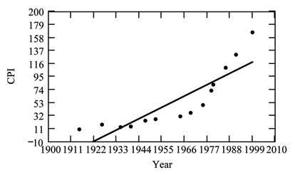
If you are interested in seeing more years of data, visit the Bureau of Labor Statistics CPI website ftp://ftp.bls.gov/pub/special.requests/cpi/cpiai.txt ; our data is taken from the column entitled "Annual Avg." (third column from the right). For example you could add more current years of data. Try adding the more recent years 2004 : CPI=188.9, 2008 : CPI=215.3 and 2011: CPI=224.9. See how it affects the model. (Check: . . Is significant? Is the fit better with the addition of the new points?)
**With contributions from Roberta Bloom
Notification Switch
Would you like to follow the 'Quantitative information analysis iii' conversation and receive update notifications?

|
|

|
|

|
|

|
|

|
|

|
|

|
|

|
|

|
|

|