13.4 Motion equations for constant acceleration in one dimension  (Page 4/8)

What else can we learn by examining the equation $x=x_0+v_{0}t+\frac{1}{2}{\text{at}}^2?$ We see that:

• displacement depends on the square of the elapsed time when acceleration is not zero. In [link] , the dragster covers only one fourth of the total distance in the first half of the elapsed time
• if acceleration is zero, then the initial velocity equals average velocity ( $v_0=\stackrel{-}{v}$ ) and $x=x_0+v_{0}t+\frac{1}{2}{\text{at}}^2$ becomes $x=x_0+v_{0}t$

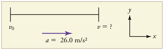
Calculating final velocity: dragsters

Calculate the final velocity of the dragster in [link] without using information about time.

Strategy

Draw a sketch.

The equation $v^2=v_0^2+2a(x-x_0)$ is ideally suited to this task because it relates velocities, acceleration, and displacement, and no time information is required.

Solution

1. Identify the known values. We know that $v_0=0$ , since the dragster starts from rest. Then we note that $x-x_0=\text{402 m}$ (this was the answer in [link] ). Finally, the average acceleration was given to be $a=\text{26}\text{.}{\text{0 m/s}}^2$ .

2. Plug the knowns into the equation $v^2=v_0^2+2a(x-x_0)$ and solve for $v.$

$v^2=0+2\left(\text{26}\text{.}{\text{0 m/s}}^2\right)\left(\text{402 m}\right).$

Thus

$v^2=2\text{.}\text{09}\times {\text{10}}^4{\text{m}}^2{\text{/s}}^2.$

To get $v$ , we take the square root:

$v=\sqrt{2\text{.}\text{09}\times {\text{10}}^4{\text{m}}^2{\text{/s}}^2}=\text{145 m/s}.$

Discussion

145 m/s is about 522 km/h or about 324 mi/h, but even this breakneck speed is short of the record for the quarter mile. Also, note that a square root has two values; we took the positive value to indicate a velocity in the same direction as the acceleration.

An examination of the equation $v^2=v_0^2+2a(x-x_0)$ can produce further insights into the general relationships among physical quantities:

• The final velocity depends on how large the acceleration is and the distance over which it acts
• For a fixed deceleration, a car that is going twice as fast doesn’t simply stop in twice the distance—it takes much further to stop. (This is why we have reduced speed zones near schools.)

Putting equations together

In the following examples, we further explore one-dimensional motion, but in situations requiring slightly more algebraic manipulation. The examples also give insight into problem-solving techniques. The box below provides easy reference to the equations needed.

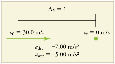
Calculating displacement: how far does a car go when coming to a halt?

On dry concrete, a car can decelerate at a rate of $7\text{.}{\text{00 m/s}}^2$ , whereas on wet concrete it can decelerate at only $5\text{.}{\text{00 m/s}}^2$ . Find the distances necessary to stop a car moving at 30.0 m/s (about 110 km/h) (a) on dry concrete and (b) on wet concrete. (c) Repeat both calculations, finding the displacement from the point where the driver sees a traffic light turn red, taking into account his reaction time of 0.500 s to get his foot on the brake.

Strategy

Draw a sketch.

In order to determine which equations are best to use, we need to list all of the known values and identify exactly what we need to solve for. We shall do this explicitly in the next several examples, using tables to set them off.