

| << Chapter < Page | Chapter >> Page > |
We then plot the results on a 2-D plane using
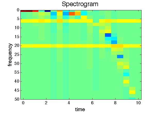
imagesc() . This function associates colors with the values in the matrix, so that you can see where the values in the matrix are larger. Thus we get a pretty picture as above.
For the first test, we will try a simple sin wave.
For the second test, we will use a more interesting function. Below we have plotted over .
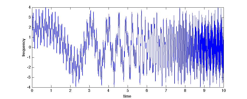
This function is interesting because it contains a frequency component that is changing over time. While we have waves at a constant 6 and 20 Hertz, the third component speeds up as gets larger and the exponential curve gets steeper. Thus for the plot we expect to see a frequency component that is increasing. This is exactly what we see in [link] –two constant bands of frequency, and one train of frequency that increases with time.
>> dt = 1e-4;>> t = 0:sr:10;>> y = sin(6*2*pi*t)+sin(20*2*pi*t)+2*sin(exp(t/1.5));>> my_stft(y, dt, 5000);
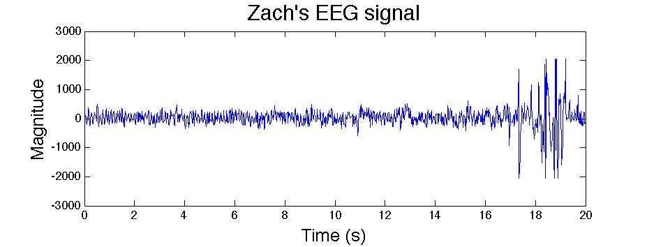
For the final section, we will analyze actual brain waves. We recorded from and EEG, and got the signal in [link] .
To analyze, we find the time-step in the data, then call mysgram(). This gives us the plot below.
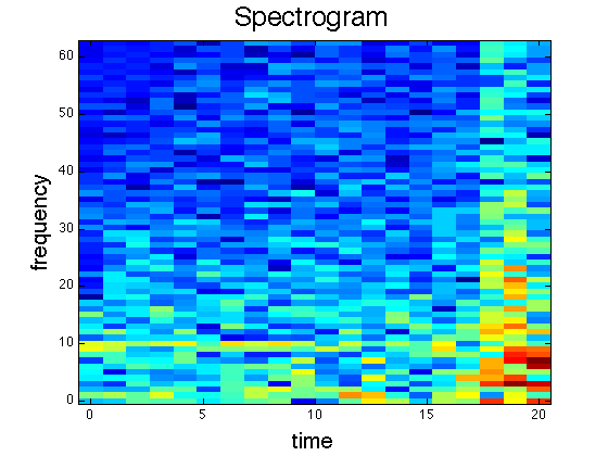
Compare the spectrogram to the raw signal. What do you notice? Perhaps the most notable change is the significant increase in signal magnitude near 18 seconds. This is reflected in the spectrogram with the brighter colors. Also, several "dominant" frequencies emerge. Two faint bands appear at 10 Hz 4 Hz for the first half of the signal. In the last section, a cluster of frequencies between 6 and 10 Hz dominate. Many of the patterns are hidden behind the subtleties in the data, however. Decoding the spectrogram is at least as difficult and creating it. Indeed, it is much less defined. The next section will explore these rules in the context of an interesting application.
One application of decoding brain waves is giving commands to a machine via brainwaves. To see developing work in this field, see this video of the company NeuroSky. Of the many machines we could command, we choose here to command a virtual car (some assembly required) that goes left or right. As above, the decision rule for such a program is not obvious. As a first try, we can find the strongest frequency for each time section and compare it to a set value. If it is lower, the car moves left, and if higher, the car moves right. The following code implements this rule:
%load dataload bwave
N = numel(eeg_sig);win_len = 3 * round(N / 60);
n = 0;freq_criterion = 8;

while (n+3) * win_len / 3<= N %for each time window
    %define the moving window and isolate that piece of signalsig_win = eeg_sig(round(n * win_len / 3) + (1:win_len));%perform fourier analysis
    [freq raw_amps]= myfourier(sig_win, dt, 1);
    %only take positive frequenciesfreq = freq((end/2+1):end);
    %add sine and cosine entries togethefamps = abs(sum(raw_amps(end/2:end,1), 2));%find the maximum one
    [a idx]= max(amps);%find the frequency corresponding to the max amplitude
    max_freq = freq(idx);%decided which way the car should move based on the max frequencyif max_freq<freq_criterion;
        fprintf('Moving left.... (fmax = %f)\n', max_freq);%this is where we put animation code
    elsefprintf('Moving right.....(fmax = %f)\n', max_freq);
        %this is where we put animation codeendpause(.5); %for dramatic effect :)
    n = n + 1;end
Notification Switch
Would you like to follow the 'The art of the pfug' conversation and receive update notifications?

|
|

|
|

|
|

|
|

|
|

|
|

|
|

|
|

|
|
|
|