

| << Chapter < Page | Chapter >> Page > |
As part of an experiment to see how different types of soil cover would affect slicing tomato production, Marist College students grew tomato plants under different soil cover conditions. Groups of three plants each had one of the following treatments
All plants grew under the same conditions and were the same variety. Students recorded the weight (in grams) of tomatoes produced by each of the n = 15 plants:
| Bare: n 1 = 3 | Ground Cover: n 2 = 3 | Plastic: n 3 = 3 | Straw: n 4 = 3 | Compost: n 5 = 3 |
|---|---|---|---|---|
| 2,625 | 5,348 | 6,583 | 7,285 | 6,277 |
| 2,997 | 5,682 | 8,560 | 6,897 | 7,818 |
| 4,915 | 5,482 | 3,830 | 9,230 | 8,677 |
Create the one-way ANOVA table.
Enter the data into lists L1, L2, L3, L4 and L5. Press STAT and arrow over to TESTS. Arrow down to ANOVA. Press ENTER and enter L1, L2, L3, L4, L5). Press ENTER. The table was filled in with the results from the calculator.
One-Way ANOVA table:
| Source of Variation | Sum of Squares ( SS ) | Degrees of Freedom ( df ) | Mean Square ( MS ) | F |
|---|---|---|---|---|
| Factor (Between) | 36,648,561 | 5 – 1 = 4 | ||
| Error (Within) | 20,446,726 | 15 – 5 = 10 | ||
| Total | 57,095,287 | 15 – 1 = 14 |
The one-way ANOVA hypothesis test is always right-tailed because larger F -values are way out in the right tail of the F -distribution curve and tend to make us reject H 0 .
Let’s return to the slicing tomato exercise in [link] . The means of the tomato yields under the five mulching conditions are represented by μ 1 , μ 2 , μ 3 , μ 4 , μ 5 . We will conduct a hypothesis test to determine if all means are the same or at least one is different. Using a significance level of 5%, test the null hypothesis that there is no difference in mean yields among the five groups against the alternative hypothesis that at least one mean is different from the rest.
The null and alternative hypotheses are:
H 0 : μ 1 = μ 2 = μ 3 = μ 4 = μ 5
H a : μ i ≠ μ j some i ≠ j
The one-way ANOVA results are shown in [link]
| Source of Variation | Sum of Squares ( SS ) | Degrees of Freedom ( df ) | Mean Square ( MS ) | F |
|---|---|---|---|---|
| Factor (Between) | 36,648,561 | 5 – 1 = 4 | ||
| Error (Within) | 20,446,726 | 15 – 5 = 10 | ||
| Total | 57,095,287 | 15 – 1 = 14 |
Distribution for the test: F 4,10
df ( num ) = 5 – 1 = 4
df ( denom ) = 15 – 5 = 10
Test statistic: F = 4.4810
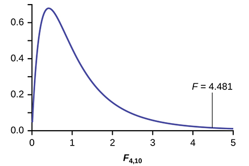
Probability Statement: p -value = P ( F >4.481) = 0.0248.
Compare α and the p -value: α = 0.05, p -value = 0.0248
Make a decision: Since α > p -value, we cannot accept H 0 .
Conclusion: At the 5% significance level, we have reasonably strong evidence that differences in mean yields for slicing tomato plants grown under different mulching conditions are unlikely to be due to chance alone. We may conclude that at least some of mulches led to different mean yields.
MRSA, or Staphylococcus aureus , can cause a serious bacterial infections in hospital patients. [link] shows various colony counts from different patients who may or may not have MRSA.
| Conc = 0.6 | Conc = 0.8 | Conc = 1.0 | Conc = 1.2 | Conc = 1.4 |
|---|---|---|---|---|
| 9 | 16 | 22 | 30 | 27 |
| 66 | 93 | 147 | 199 | 168 |
| 98 | 82 | 120 | 148 | 132 |
Plot of the data for the different concentrations:
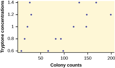
Test whether the mean number of colonies are the same or are different. Construct the ANOVA table, find the p -value, and state your conclusion. Use a 5% significance level.
While there are differences in the spreads between the groups (see [link] ), the differences do not appear to be big enough to cause concern.
We test for the equality of mean number of colonies:
H a : μ i ≠ μ j some i ≠ j
The one-way ANOVA table results are shown in [link] .
| Source of Variation | Sum of Squares ( SS ) | Degrees of Freedom ( df ) | Mean Square ( MS ) | F |
|---|---|---|---|---|
| Factor (Between) | 10,233 | 5 – 1 = 4 | ||
| Error (Within) | 41,949 | 15 – 5 = 10 | ||
| Total | 52,182 | 15 – 1 = 14 |
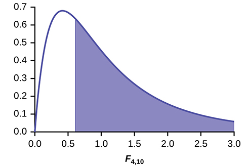
Distribution for the test: F 4,10
Probability Statement: p -value = P ( F >0.6099) = 0.6649.
Compare α and the p -value: α = 0.05, p -value = 0.669, α > p -value
Make a decision: Since α > p -value, we do not reject H 0 .
Conclusion: At the 5% significance level, there is insufficient evidence from these data that different levels of tryptone will cause a significant difference in the mean number of bacterial colonies formed.
Notification Switch
Would you like to follow the 'Introductory statistics' conversation and receive update notifications?

|
|

|
|

|
|

|
|

|
|

|
|

|
|

|
|
|
|
|

|