

| << Chapter < Page | Chapter >> Page > |
To determine the critical points we have to find F α , df1 , df2 . See Appendix A for the F table. The F distribution has two different degrees of freedom, one associated with the numerator, df1 , and one associated with the denominator, df2 and to complicate matters the F distribution is not symmetrical and changes the degree of skewness as he degrees of freedom change. The degrees of freedom in the numerator is n 1 -1, where n 1 is the sample size for group 1, and the degrees of freedom in the denominator is n 2 -1, where n 2 is the sample size for group 2. F α , df1 , df2 will give the critical value on the upper end of the F distribution.
To find the critical value for the lower end of the distribution, reverse the degrees of freedom and divide the F-value into one.
When the calculated value of F is between the critical values we cannot reject the null hypothesis that the two variances came from a population with the same variance. If the calculated F-value is in either tail we cannot accept the null hypothesis just as we have been doing for all of the previous tests of hypothesis.
An alternative way of finding the critical values of the F distribution makes the use of the F-table easier. We note on the F-table that all the values of F are greater than one therefore the critical F value for the left hand tail will always be less than one because to find the critical value on the left tail we divide an F value into the number one. We also note that if the sample standard deviation in the numerator of the test statistic is larger than the sample standard deviation in the denominator, the resulting F value will be greater than one. The shorthand method for this test is thus to be sure that the larger of the two sample standard deviations is placed in the numerator to calculate the test statistic. This will mean that only the right had tail critical value will have to be found in the F-table.
Two college instructors are interested in whether or not there is any variation in the way they grade math exams. They each grade the same set of 30 exams. The first instructor's grades have a variance of 52.3. The second instructor's grades have a variance of 89.9. Test the claim that the first instructor's variance is smaller. (In most colleges, it is desirable for the variances of exam grades to be nearly the same among instructors.) The level of significance is 10%.
Let 1 and 2 be the subscripts that indicate the first and second instructor, respectively.
n 1 = n 2 = 30.
H 0 : and H a :
Calculate the test statistic: By the null hypothesis , the F statistic is:
Critical value for the test: F 29,29 where n 1 – 1 = 29 and n 2 – 1 = 29 = 1.65.
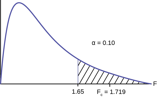
Make a decision: Since the calculated F value is not in the tail we cannot accept H 0 .
Conclusion: With a 10% level of significance, from the data, there is sufficient evidence to conclude that the variance in grades for the first instructor is smaller.
The New York Choral Society divides male singers up into four categories from highest voices to lowest: Tenor1, Tenor2, Bass1, Bass2. In the table are heights of the men in the Tenor1 and Bass2 groups. One suspects that taller men will have lower voices, and that the variance of height may go up with the lower voices as well. Do we have good evidence that the variance of the heights of singers in each of these two groups (Tenor1 and Bass2) are different?
| Tenor1 | Bass2 | Tenor 1 | Bass 2 | Tenor 1 | Bass 2 |
|---|---|---|---|---|---|
| 69 | 72 | 67 | 72 | 68 | 67 |
| 72 | 75 | 70 | 74 | 67 | 70 |
| 71 | 67 | 65 | 70 | 64 | 70 |
| 66 | 75 | 72 | 66 | 69 | |
| 76 | 74 | 70 | 68 | 72 | |
| 74 | 72 | 68 | 75 | 71 | |
| 71 | 72 | 64 | 68 | 74 | |
| 66 | 74 | 73 | 70 | 75 | |
| 68 | 72 | 66 | 72 |
The histograms are not as normal as one might like. Plot them to verify. However, we proceed with the test in any case.
Subscripts: T1= tenor1 and B2 = bass 2
The standard deviations of the samples are s T 1 = 3.3302 and s B 2 = 2.7208.
The hypotheses are
and (two tailed test)
The F statistic is 1.4894 with 20 and 25 degrees of freedom.
The p -value is 0.3430. If we assume alpha is 0.05, then we cannot reject the null hypothesis.
We have no good evidence from the data that the heights of Tenor1 and Bass2 singers have different variances (despite there being a significant difference in mean heights of about 2.5 inches.)
Notification Switch
Would you like to follow the 'Introductory statistics' conversation and receive update notifications?

|
|

|
|

|
|

|
|

|
|

|
|

|
|

|
|

|
|

|