This module provides an overview of Linear Regression and Correlation: The Correlation Coefficient and Coefficient of Determination. It is part of the Roberta Bloom's Custom Collection of Collaborative Statistics (col10617). It is based on module m17092 as a part of Collaborative Statistics collection (col10522) by Barbara Illowsky and Susan Dean. This revised has been expanded from the original to include coverage of the coefficient of determination and to include a discussion of properties of the correlation coefficient previously included in Illowsky and Dean's module. Some material previously in module m17077 Facts about the Correlation Coefficient have been moved to this module in Bloom's custom edition of Collaborative Statistics.
The correlation coefficient r
Besides looking at the scatter plot and seeing that a line seems reasonable, how can you
tell if the line is a good predictor? Use the correlation coefficient as another indicator(besides the scatterplot) of the strength of the relationship between
and
.
The
correlation coefficient, r, developed by Karl Pearson in the early 1900s, is a numerical measure of the strength of association between the independent variable x and the dependent variable y.
The correlation coefficient is calculated as
where
= the number of data points.
If you suspect a linear relationship between
and
, then
can measure how strong the linear relationship is.
What the value of r tells us:
The value of
is always between -1 and +1:
.
The closer the correlation coefficient
is to -1 or 1 (and the further from 0), the stronger the evidence of a significant linear relationship between
and
; this would indicate that the observed data points fit more closely to the best fit line. Values of
further from 0 indicate a stronger linear relationship between
and
. Values of
closer to 0 indicate a weaker linear relationship between
and
.
If
there is absolutely no linear relationship between
and
(no linear correlation) .
If
, there is perfect positive correlation. If
, there is perfect negative
correlation. In both these cases, all of the original data points lie on a straight line. Of course,in the real world, this will not generally happen.
What the sign of r tells us
A positive value of
means that when
increases,
increases and when
decreases,
decreases
(positive correlation) .
A negative value of
means that when
increases,
decreases and when
decreases,
increases
(negative correlation) .
The sign of
is the same as the sign of the slope,
,
of the best fit line.
Strong correlation does not suggest that
causes
or
causes
. We say
"correlation does not imply causation." For example, every person who learned
math in the 17th century is dead. However, learning math does not necessarily causedeath!
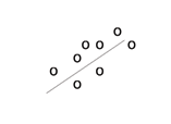
Positive correlation
A scatter plot showing data with a positive correlation.
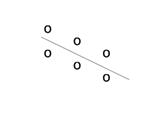
Negative correlation
A scatter plot showing data with a negative correlation.
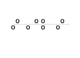
Zero correlation
A scatter plot showing data with zero correlation.
=0
The formula for
looks formidable. However, computer spreadsheets, statistical software, and many calculators can quickly calculate
. The correlation coefficient
is the bottom item in the output screens for the LinRegTTest on the TI-83, TI-83+, or TI-84+ calculator (see previous section for instructions).
The coefficient of determination
is called the coefficient of determination.
is the square of the correlation coefficient , but is usually stated as a percent, rather than in decimal form.
has an interpretation in the context of the data
, when expressed as a percent, represents the percent of variation in the dependent variable y that can be explained by variation in the independent variable x using the regression (best fit) line.
1-
, when expressed as a percent, represents the percent of variation in y that is NOT explained by variation in x using the regression line. This can be seen as the scattering of the observed data points about the regression line.
Approximately 44% of the variation in the final exam grades can be explained by the variation in the grades on the third exam, using the best fit regression line.
Therefore approximately 56% of the variation in the final exam grades can NOT be explained by the variation in the grades on the third exam, using the best fit regression line. (This is seen as the scattering of the points about the line.)
In the next section, we will learn more about the correlation coefficient and will examine
in the context of the example about grades on the third exam and final exam.
Receive real-time job alerts and never miss the right job again
Source:
OpenStax, Collaborative statistics: custom version modified by v moyle. OpenStax CNX. Nov 14, 2010 Download for free at http://legacy.cnx.org/content/col11238/1.2
Google Play and the Google Play logo are trademarks of Google Inc.
Notification Switch
Would you like to follow the 'Collaborative statistics: custom version modified by v moyle' conversation and receive update notifications?