

| << Chapter < Page | Chapter >> Page > |
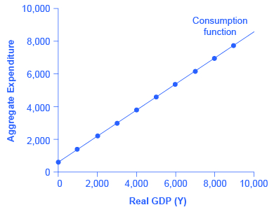
The pattern of consumption shown in [link] is plotted in [link] . To calculate consumption, multiply the income level by 0.8, for the marginal propensity to consume, and add $600, for the amount that would be consumed even if income was zero. Consumption plus savings must be equal to income.
| Income | Consumption | Savings |
|---|---|---|
| $0 | $600 | –$600 |
| $1,000 | $1,400 | –$400 |
| $2,000 | $2,200 | –$200 |
| $3,000 | $3,000 | $0 |
| $4,000 | $3,800 | $200 |
| $5,000 | $4,600 | $400 |
| $6,000 | $5,400 | $600 |
| $7,000 | $6,200 | $800 |
| $8,000 | $7,000 | $1,000 |
| $9,000 | $7,800 | $1,200 |
However, a number of factors other than income can also cause the entire consumption function to shift. These factors were summarized in the earlier discussion of consumption, and listed in [link] . When the consumption function moves, it can shift in two ways: either the entire consumption function can move up or down in a parallel manner, or the slope of the consumption function can shift so that it becomes steeper or flatter. For example, if a tax cut leads consumers to spend more, but does not affect their marginal propensity to consume, it would cause an upward shift to a new consumption function that is parallel to the original one. However, a change in household preferences for saving that reduced the marginal propensity to save would cause the slope of the consumption function to become steeper: that is, if the savings rate is lower, then every increase in income leads to a larger rise in consumption.
Investment decisions are forward-looking, based on expected rates of return. Precisely because investment decisions depend primarily on perceptions about future economic conditions, they do not depend primarily on the level of GDP in the current year. Thus, on a Keynesian cross diagram, the investment function can be drawn as a horizontal line, at a fixed level of expenditure. [link] shows an investment function where the level of investment is, for the sake of concreteness, set at the specific level of 500. Just as a consumption function shows the relationship between consumption levels and real GDP (or national income), the investment function shows the relationship between investment levels and real GDP.

Notification Switch
Would you like to follow the 'Principles of macroeconomics for ap® courses' conversation and receive update notifications?

|
|
|
|
|

|
|

|
|

|
|

|
|

|
|

|
|

|
|

|
|

|
|

|