10.3 Problems on functions of random variables (Page 3/3)

Applied probability Page 3 / 3

$f_{X Y} (t, u) = \frac{3}{88} (2 t + 3 u^{2})$ for $0 \leq t \leq 2$ , $0 \leq u \leq 1 + t$ (see Exercise 15 from "Problems on Random Vectors and Joint Distributions").

Z = I_{[0, 1]} (X) 4 X + I_{(1, 2]} (X) (X + Y)

Determine $P (Z \leq 2)$

P (Z \leq 2) = P (Z \in Q = Q 1 M 1 ⋁ Q 2 M 2), where M 1 = {(t, u) : 0 \leq t \leq 1, 0 \leq u \leq 1 + t}

M 2 = {(t, u) : 1 < t \leq 2, 0 \leq u \leq 1 + t}

Q 1 = {(t, u) : 0 \leq t \leq 1 / 2}, Q 2 = {(t, u) : u \leq 2 - t} (see figure)

P = \frac{3}{88} \int_{0}^{1 / 2} \int_{0}^{1 + t} (2 t + 3 u^{2}) d u d t + \frac{3}{88} \int_{1}^{2} \int_{0}^{2 - t} (2 t + 3 u^{2}) d u d t = \frac{563}{5632}

tuappr
Enter matrix [a b]of X-range endpoints  [0 2]
Enter matrix [c d]of Y-range endpoints  [0 3]
Enter number of X approximation points  200Enter number of Y approximation points  300
Enter expression for joint density  (3/88)*(2*t + 3*u.^2).*(u<=1+t)
Use array operations on X, Y, PX, PY, t, u, and PG = 4*t.*(t<=1) + (t+u).*(t>1);
[Z,PZ]= csort(G,P);
PZ2 = (Z<=2)*PZ'
PZ2 =  0.1010                       % Theoretical = 563/5632 = 0.1000

Got questions? Get instant answers now!

Figure 1 is comprised of two separate figures, one for exercise 11, on the left, and one for exercise 12, on the right. The figure for exercise 11 is a cartesian graph of the first quadrant, with the horizontal axis labeled t, and the vertical axis labeled u. The values on the horizontal axis range from 0 to 2, in increments of 1, with an extra marking in between 0 and 1 for the value 0.5. The values on the vertical axis range from 0 to 3 in increments of 1. The figure contains three major shapes, with two smaller shaded shapes located inside a larger polygon. The large polygon has four sides. The first is a vertical portion located on the vertical axis, from (0, 0) to (0, 1). The upper side is a diagonal line, labeled u = 1 + t, that is drawn from (0, 1) to (2, 3). The rightmost side is another vertical line from the end of the second side at (2, 3) to the horizontal axis, at (2, 0). The bottom side of the shape connects (2, 0) horizontally to the origin, completing the shape. Inside this large polygon are two shaded shapes. The first is a right triangle with right-angle vertex located at (1, 0). One side is drawn vertically from (1, 0) to (1, 1), another is drawn horizontally from (1, 0) to (2, 0), and the hypotenuse is connected from (1, 1) to (2, 0). The hypotenuse is labeled u = 2 - t. There is a dashed vertical line connecting the triangles vertex at (1, 1) to the midpoint of the large polygon's diagonal side, at (1, 2). The second small shape is similar to the large polygon. It shares the same side on the vertical axis from (0, 0) to (0,1), and shares a portion of the diagonal line u = 1 + t from (0, 1) to (0.5, 1.5). Its third side is drawn vertically from that point to (0.5, 0) on the horizontal axis. A fourth side completes the polygon from (0.5, 0) to the origin. The figure for exercise 12 is a cartesian graph of the first quadrant, with the horizontal axis labeled t, and the vertical axis labeled u. The values on the horizontal axis range from 0 to 2, in increments of 1, with an extra marking for the value 0.5. The vertical axis does not contain any markings for values. There are five lines, which, connecting to the horizontal and vertical axes, create four separate enclosed sections. Two of these sections are shaded. The outermost lines are labeled with equations. A horizontal line from (0, 1) to (1, 1) is labeled u = 1. A diagonal line with negative slope connects to the horizontal line and the t-axis from (1, 1) to (2, 0) and is labeled u = 2 - t. These two labeled lines, along with the u and t-axes, create a four-sided polygon with two horizontal sides, one vertical side on the u-axis, and one diagonal side of negative slope labeled u = 2 - t. There are three interior lines. The longest interior line extends from the origin to point (1, 1), and in doing so, divides the larger aforementioned polygon into two triangles. The first smaller interior line is drawn from (0.5, 1) to (0.5, 0.5), a vertical line. The second is drawn from (0.5, 0.5) to approximately (1.5, 0.5) a horizontal line. These two smaller interior lines divide the two aforementioned triangles into two smaller triangles, a large symmetric trapezoid, and a four-sided polygon. The polygon inside and the trapezoid are shaded, and the smaller triangles remain white.

$f_{X Y} (t, u) = \frac{24}{11} t u$ for $0 \leq t \leq 2$ , $0 \leq u \leq min {1, 2 - t}$ (see Exercise 17 from "Problems on Random Vectors and Joint Distributions").

Z = I_{M} (X, Y) \frac{1}{2} X + I_{M^{c}} (X, Y) Y^{2}, M = {(t, u) : u > t}

Determine $P (Z \leq 1 / 4)$ .

P (Z \leq 1 / 4) = P ((X, Y) \in M_{1} Q_{1} ⋁ M_{2} Q_{2}), M_{1} = {(t, u) : 0 \leq t \leq u \leq 1}

M_{2} = {(t, u) : 0 \leq t \leq 2, 0 \leq t \leq min (t, 2 - t)}

Q_{1} = {(t, u) : t \leq 1 / 2} Q_{2} = {(t, u) : u \leq 1 / 2} (see figure)

P = \frac{24}{11} \int_{0}^{1 / 2} \int_{0}^{1} t u d u d t + \frac{24}{11} \int_{1 / 2}^{3 / 2} \int_{0}^{1 / 2} t u d u d t + \frac{24}{11} \int_{3 / 2}^{2} \int_{0}^{2 - t} t u d u d t = \frac{85}{176}

tuappr
Enter matrix [a b]of X-range endpoints  [0 2]
Enter matrix [c d]of Y-range endpoints  [0 1]
Enter number of X approximation points  400Enter number of Y approximation points  200
Enter expression for joint density  (24/11)*t.*u.*(u<=min(1,2-t))
Use array operations on X, Y, PX, PY, t, u, and PG = 0.5*t.*(u>t) + u.^2.*(u<t);
[Z,PZ]= csort(G,P);
pp = (Z<=1/4)*PZ'
pp =  0.4844                        % Theoretical = 85/176 = 0.4830

Got questions? Get instant answers now!

$f_{X Y} (t, u) = \frac{3}{23} (t + 2 u)$ for $0 \leq t \leq 2$ , $0 \leq u \leq max {2 - t, t}$ (see Exercise 18 from "Problems on Random Vectors and Joint Distributions").

Z = I_{M} (X, Y) (X + Y) + I_{M^{c}} (X, Y) 2 Y, M = {(t, u) : max (t, u) \leq 1}

Determine $P (Z \leq 1)$ .

P (Z \leq 1) = P ((X, Y) \in M_{1} Q_{1} ⋁ M_{2} Q_{2}), M_{1} = {(t, u) : 0 \leq t \leq 1, 0 \leq u \leq 1 - t}

M_{2} = {(t, u) : 1 \leq t \leq 2, 0 \leq u \leq t}

Q_{1} = {(t, u) : u \leq 1 - t} Q_{2} = {(t, u) : u \leq 1 / 2} (see figure)

P = \frac{3}{23} \int_{0}^{1} \int_{0}^{1 - t} (t + 2 u) d u d t + \frac{3}{23} \int_{1}^{2} \int_{0}^{1 / 2} (t + 2 u) d u d t = \frac{9}{46}

tuappr
Enter matrix [a b]of X-range endpoints  [0 2]
Enter matrix [c d]of Y-range endpoints  [0 2]
Enter number of X approximation points  300Enter number of Y approximation points  300
Enter expression for joint density  (3/23)*(t + 2*u).*(u<=max(2-t,t))
Use array operations on X, Y, PX, PY, t, u, and PM = max(t,u)<= 1;
G = M.*(t + u) + (1 - M)*2.*u;p = total((G<=1).*P)
p =  0.1960                         % Theoretical = 9/46 = 0.1957

Got questions? Get instant answers now!

Figure two is comprised of two cartesian graphs, both displaying only the first coordinate. Both graphs use t as the horizontal axis and u as the vertical axis. Both axes on the graphs range in value from 0 to 2 in increments of 1. The first graph, for exercise 13, contains five labeled lines, and two unlabeled lines. The lines are labeled with their equations. From (0, 2) to (1, 1) is a line segment labeled u = 2 - t. From (1, 1) to (2, 2) is a line segment labeled u = t. From (0, 1) to (1, 0) is a line segment labeled u = 1 - t. From (1, 0.5) to (2, 0.5) is a line segment labeled u = 0.5. From (2, 0) to (2, 2) is a line labeled t = 2. From (0, 1) to (1, 1) is an unlabeled line segment. From (1, 0) to (1, 1) is the final unlabeled line segment. Two shapes created by the lines on this graph are shaded. The first is a right triangle bound by u = 1 - t and the horizontal and vertical axes. The second is a rectangle bound by u = 0.5, t = 2, the vertical unlabeled line segment from (1, 0) to (1, 1), and the horizontal axis. The second graph, for exercise 14, contains 5 labeled line segments, one unlabeled line segment, and one dashed, unlabeled line segment. From (0, 2) to (1, 2) is a line segment labeled u = 2. From (0, 2) to (1, 1) is a line segment labeled u = 2 - t. From (1, 2) to (2, 1) is a line segment labeled u = 3 - t. From (1, 1) to (2, 1) is a line segment labeled u = 1. From (2, 1) to (2, 0) is a line segment labeled t = 2. The unlabeled solid line segment is drawn from (1, 2) to (1, 1). The unlabeled dashed line segment is drawn from (0, 1) to (1, 1). A large region, bounded by u = 2 - t, u = 1, t = 2, the vertical axis, and the horizontal axis, is shaded grey.

$f_{X Y} (t, u) = \frac{12}{179} (3 t^{2} + u)$ , for $0 \leq t \leq 2$ , $0 \leq u \leq min {2, 3 - t}$ (see Exercise 19 from "Problems on Random Vectors and Joint Distributions").

Z = I_{M} (X, Y) (X + Y) + I_{M^{c}} (X, Y) 2 Y^{2}, M = {(t, u) : t \leq 1, u \geq 1}

Determine $P (Z \leq 2)$ .

P (Z \leq 2) = P ((, Y) \in M_{1} Q_{1} ⋁ (M_{2} ⋁ M_{3}) Q_{2}), M_{1} = {(t, u) : 0 \leq t \leq 1, 1 \leq u \leq 2}

M_{2} = {(t, u) : 0 \leq t \leq 1, 0 \leq u \leq 1} M_{3} = {(t, u) : 1 \leq t \leq 2, 0 \leq u \leq 3 - t}

Q_{1} = {(t, u) : u \leq 1 - t} Q_{2} = {(t, u) : u \leq 1 / 2} (see figure)

P = \frac{12}{179} \int_{0}^{1} \int_{0}^{2 - t} (3 t^{2} + u) d u d t + \frac{12}{179} \int_{1}^{2} \int_{0}^{1} (3 t^{2} + u) d u d t = \frac{119}{179}

tuappr
Enter matrix [a b]of X-range endpoints  [0 2]
Enter matrix [c d]of Y-range endpoints  [0 2]
Enter number of X approximation points  300Enter number of Y approximation points  300
Enter expression for joint density  (12/179)*(3*t.^2 + u).*(u<=min(2,3-t))
Use array operations on X, Y, PX, PY, t, u, and PM = (t<=1)&(u>=1);
Z = M.*(t + u) + (1 - M)*2.*u.^2;G = M.*(t + u) + (1 - M)*2.*u.^2;
p = total((G<=2).*P)
p =  0.6662                          % Theoretical = 119/179 = 0.6648

Got questions? Get instant answers now!

$f_{X Y} (t, u) = \frac{12}{227} (3 t + 2 t u)$ , for $0 \leq t \leq 2$ , $0 \leq u \leq min {1 + t, 2}$ (see Exercise 20 from "Problems on Random Variables and Joint Distributions")

Z = I_{M} (X, Y) X + I_{M^{c}} (X, Y) \frac{Y}{X}, M = {(t, u) : u \leq min (1, 2 - t)}

Detemine $P (Z \leq 1)$ .

Figure three, for exercise 15, is comprised of one cartesian graph, with only the first quadrant displayed. The horizontal axis is labeled t, and the vertical axis is labeled u. The values on both axes range from 0 to 2 in increments of 1. There are 6 labeled line segments, one unlabeled line segment, and two resulting shaded shapes in this figure. The line segment from (0, 1) to (1, 2) is labeled u = 1 + t. The line segment from (0, 1) to (1, 1) is labeled u = 1. The line segment from (1, 2) to (2, 2) is labeled u = 2. The line segment from (1, 1) to (2, 2) is labeled u = t. The line segment from (1, 1) to (2, 0) is labeled u = 2 - t. The line segment from (2, 0) to (2, 2) is labeled t = 2. The unlabeled line segment is drawn from (1, 0) to (1, 1). A shaded square resulting from the drawn segments is bound by u = 1, the vertical axis, the horizontal axis, and the unlabeled line segment. A shaded triangle is bound by u = t, u = 2 - t, and t = 2.

P (Z \leq 1) = P ((X, Y) \in M_{1} Q_{1} ⋁ M_{2} Q_{2}), M_{1} = M, M_{2} = M^{c}

Q_{1} = {(t, u) : 0 \leq t \leq 1} Q_{2} = {(t, u) : u \leq t} (see figure)

P = \frac{12}{227} \int_{0}^{1} \int_{0}^{1} (3 t + 2 t u) d u d t + \frac{12}{227} \int_{1}^{2} \int_{2 - t}^{t} (3 t + 2 t u) d u d t = \frac{124}{227}

tuappr
Enter matrix [a b]of X-range endpoints  [0 2]
Enter matrix [c d]of Y-range endpoints  [0 2]
Enter number of X approximation points  400Enter number of Y approximation points  400
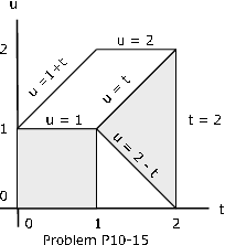
Enter expression for joint density  (12/227)*(3*t+2*t.*u).*(u<=min(1+t,2))
Use array operations on X, Y, PX, PY, t, u, and PQ = (u<=1).*(t<=1) + (t>1).*(u>=2-t).*(u<=t);
P = total(Q.*P)P =  0.5478                        % Theoretical = 124/227 = 0.5463

Got questions? Get instant answers now!

The class ${X, Y, Z}$ is independent.

$X = - 2 I_{A} + I_{B} + 3 I_{C}$ . Minterm probabilities are (in the usual order)

0.255 0.025 0.375 0.045 0.108 0.012 0.162 0.018

$Y = I_{D} + 3 I_{E} + I_{F} - 3$ . The class ${D, E, F}$ is independent with

P (D) = 0.32 P (E) = 0.56 P (F) = 0.40

Z has distribution

Value	-1.3	1.2	2.7	3.4	5.8
Probability	0.12	0.24	0.43	0.13	0.08

Determine $P (X^{2} + 3 X Y^{2} > 3 Z)$ .

% file
npr10_16.m Data for
[link] cx = [-2 1 3 0];pmx = 0.001*[255  25 375  45 108  12 162  18];cy = [1 3 1 -3];pmy = minprob(0.01*[32 56 40]);Z = [-1.3 1.2 2.7 3.4 5.8];PZ = 0.01*[12 24 43 13  8];disp('Data are in cx, pmx, cy, pmy, Z, PZ')
npr10_16                % Call for dataData are in cx, pmx, cy, pmy, Z, PZ
[X,PX]= canonicf(cx,pmx);
[Y,PY]= canonicf(cy,pmy);
icalc3Enter row matrix of X-values  X
Enter row matrix of Y-values  YEnter row matrix of Z-values  Z
Enter X probabilities  PXEnter Y probabilities  PY
Enter Z probabilities  PZUse array operations on matrices X, Y, Z,
PX, PY, PZ, t, u, v, and PM = t.^2 + 3*t.*u.^2>3*v;
PM = total(M.*P)PM =  0.3587

Got questions? Get instant answers now!

The simple random variable X has distribution

X = [- 3.1 - 0.5 1.2 2.4 3.7 4.9] P X = [0.15 0.22 0.33 0.12 0.11 0.07]

Plot the distribution function F _X and the quantile function Q _X .
Take a random sample of size $n = 10, 000$ . Compare the relative frequency for each value with the probability that value is taken on.

X = [-3.1 -0.5 1.2 2.4 3.7 4.9];PX = 0.01*[15 22 33 12 11  7];ddbn
Enter row matrix of VALUES  XEnter row matrix of PROBABILITIES  PX  % Plot not reproduced here
dquanplotEnter VALUES for X  X
Enter PROBABILITIES for X  PX          % Plot not reproduced hererand('seed',0)                      % Reset random number generator
dsample                             % for comparison purposesEnter row matrix of VALUES  X
Enter row matrix of PROBABILITIES  PXSample size n  10000
    Value      Prob    Rel freq-3.1000    0.1500    0.1490
   -0.5000    0.2200    0.21641.2000    0.3300    0.3340
    2.4000    0.1200    0.11843.7000    0.1100    0.1070
    4.9000    0.0700    0.0752Sample average ex = 0.8792
Population mean E[X]= 0.859
Sample variance vx = 5.146Population variance Var[X] = 5.112

Got questions? Get instant answers now!

<< Chapter < Page Page > Chapter >>

Read also:

Get Jobilize Job Search Mobile App in your pocket Now!

100% Free Mobile Applications
Receive real-time job alerts and never miss the right job again

Source: OpenStax, Applied probability. OpenStax CNX. Aug 31, 2009 Download for free at http://cnx.org/content/col10708/1.6

Google Play and the Google Play logo are trademarks of Google Inc.

Notification Switch

Would you like to follow the 'Applied probability' conversation and receive update notifications?

Ask

	22 AP Key Terms 22 The Respiratory System By OpenStax Start Key Terms
	47 Biology 47 Conservation Biology Biodiversity MCQ By OpenStax Start Quiz
	6 AP Key Terms 06 The Skeletal System By OpenStax Start Key Terms
©flickr:	Morphology By Jugnu Khan Start Quiz
	2 Gastrointestinal Pathophysiology Self-Assessment By Laurence Bailen Start Assessment
	Capitalism Market Economy By Robert Murphy Start Test
	2 Biology 02 The Chemical Foundation of Life MCQ By OpenStax Start Quiz
	3 Arts Society: Theater 3 By Jonathan Long Start Quiz
©flickr: Gareth	Professional Etiquette MCQ By Abby Sharp Start Quiz
	OOP with Java - Quiz 1 By Vongkol HENG Start Quiz