

| << Chapter < Page | Chapter >> Page > |
| Labor | Quantity | Fixed Cost | Variable Cost | Total Cost |
|---|---|---|---|---|
| 1 | 16 | $160 | $80 | $240 |
| 2 | 40 | $160 | $160 | $320 |
| 3 | 60 | $160 | $240 | $400 |
| 4 | 72 | $160 | $320 | $480 |
| 5 | 80 | $160 | $400 | $560 |
| 6 | 84 | $160 | $480 | $640 |
| 7 | 82 | $160 | $560 | $720 |
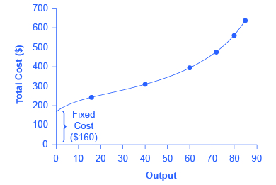
The relationship between the quantity of output being produced and the cost of producing that output is shown graphically in the figure. The fixed costs are always shown as the vertical intercept of the total cost curve; that is, they are the costs incurred when output is zero so there are no variable costs.
You can see from the graph that once production starts, total costs and variable costs rise. While variable costs may initially increase at a decreasing rate, at some point they begin increasing at an increasing rate. This is caused by diminishing marginal returns, discussed in the chapter on Choice in a World of Scarcity , which is easiest to see with an example. As the number of barbers increases from zero to one in the table, output increases from 0 to 16 for a marginal gain of 16; as the number rises from one to two barbers, output increases from 16 to 40, a marginal gain of 24. From that point on, though, the marginal gain in output diminishes as each additional barber is added. For example, as the number of barbers rises from two to three, the marginal output gain is only 20; and as the number rises from three to four, the marginal gain is only 12.
To understand the reason behind this pattern, consider that a one-man barber shop is a very busy operation. The single barber needs to do everything: say hello to people entering, answer the phone, cut hair, sweep up, and run the cash register. A second barber reduces the level of disruption from jumping back and forth between these tasks, and allows a greater division of labor and specialization. The result can be greater increasing marginal returns. However, as other barbers are added, the advantage of each additional barber is less, since the specialization of labor can only go so far. The addition of a sixth or seventh or eighth barber just to greet people at the door will have less impact than the second one did. This is the pattern of diminishing marginal returns. As a result, the total costs of production will begin to rise more rapidly as output increases. At some point, you may even see negative returns as the additional barbers begin bumping elbows and getting in each other’s way. In this case, the addition of still more barbers would actually cause output to decrease, as shown in the last row of [link] .
This pattern of diminishing marginal returns is common in production. As another example, consider the problem of irrigating a crop on a farmer’s field. The plot of land is the fixed factor of production, while the water that can be added to the land is the key variable cost. As the farmer adds water to the land, output increases. But adding more and more water brings smaller and smaller increases in output, until at some point the water floods the field and actually reduces output. Diminishing marginal returns occur because, at a given level of fixed costs, each additional input contributes less and less to overall production.
Notification Switch
Would you like to follow the 'Openstax microeconomics in ten weeks' conversation and receive update notifications?

|
|

|
|

|
|

|
|
|
|
|
|
|
|

|
|

|
|

|
|

|