<< Chapter < Page Chapter >> Page >

Several other important properties of the quantile function may be established.

Figure 1 consists of three graphs. The first is a plot of U = F(t) with t on the horizontal axis, and u on the vertical axis. The plotted curve begins at the point (-1, 0), and increases at a constant slope until t=1. The curve then increases exponentially, beginning with a very shallow slope and increasing in slope to be nearly vertical. At t=3, the curve is cut short and a horizontal line continues to t=4. The horizontal segment is met with a vertical line segment until the curve reaches u=1, at which it again continues horizontally to the right. The second graph is identical in shape to the first graph, except that the graph moves in the downward instead of upward. The third graph plots u on the horizontal axis and t on the vertical axis, plotting t = Q(u). The curve is identical to the curve in the first graph, except with the adjusted axes, the curve is rotated 90 degrees counter-clockwise. There is also a vertical dashed line along u=1 that meets the curve at its rightmost segment. Figure 1 consists of three graphs. The first is a plot of U = F(t) with t on the horizontal axis, and u on the vertical axis. The plotted curve begins at the point (-1, 0), and increases at a constant slope until t=1. The curve then increases exponentially, beginning with a very shallow slope and increasing in slope to be nearly vertical. At t=3, the curve is cut short and a horizontal line continues to t=4. The horizontal segment is met with a vertical line segment until the curve reaches u=1, at which it again continues horizontally to the right. The second graph is identical in shape to the first graph, except that the graph moves in the downward instead of upward. The third graph plots u on the horizontal axis and t on the vertical axis, plotting t = Q(u). The curve is identical to the curve in the first graph, except with the adjusted axes, the curve is rotated 90 degrees counter-clockwise. There is also a vertical dashed line along u=1 that meets the curve at its rightmost segment.
Graph of quantile function from graph of distribution function,
  1. Q is left-continuous, whereas F is right-continuous.
  2. If jumps are represented by vertical line segments, construction of the graph of u = Q ( t ) may be obtained by the following two step procedure:
    • Invert the entire figure (including axes), then
    • Rotate the resulting figure 90 degrees counterclockwise
    This is illustrated in [link] . If jumps are represented by vertical line segments, then jumps go into flat segments and flat segments go into vertical segments.
  3. If X is discrete with probability p i at t i , 1 i n , then F has jumps in the amount p i at each t i and is constant between. The quantile function is a left-continuous step function having value t i on the interval ( b i - 1 , b i ] , where b 0 = 0 and b i = j = 1 i p j . This may be stated
    If F ( t i ) = b i , then Q ( u ) = t i for F ( t i - 1 ) < u F ( t i )

Quantile function for a simple random variable

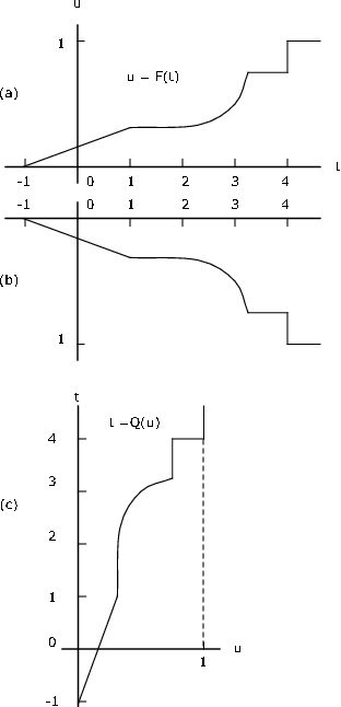
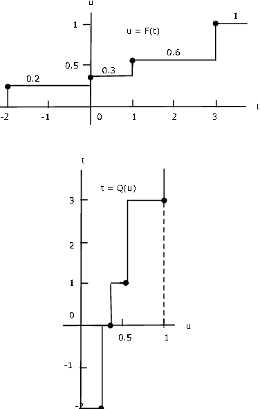
Suppose simple random variable X has distribution

X = [ - 2 0 1 3 ] P X = [ 0 . 2 0 . 1 0 . 3 0 . 4 ]

Figure 1 shows a plot of the distribution function F X . It is reflected in the horizontal axis then rotated counterclockwise to give the graph of Q ( u ) versus u .

Figure 2 consists of two graphs. The first is a plot of U = F(t) graphed with t as the horizontal axis and u as the vertical axis, starting at (-2, 0) with a small vertical segment that meets a black dot at a right angle. Continuing to the right, the line after the black dot is drawn to the vertical axis, with the number 0.2 labeled above the horizontal segment. At the vertical axis a small vertical line along the axis continues to another black dot on the vertical axis. After the black dot towards the right is another horizontal line with the number 0.3 labeled above the segment. At t=1, the horizontal segment ends, then moving vertically to a third black dot. The next segment of the plot is horizontal, extending from t=1 to t-3, labeled as 0.6. At t=3 the plot moves vertically to a fourth black dot at point (3, 1). The segment after the black dot moves horizontally to the right edge of the graph, labeled as 1. The second graph is a plot of t = Q(u), with u as the horizontal axis and t as the vertical axis. The plot is identical in shape to the plot in the first graph of figure 2 except rotated in the fashion as the axes. Figure 2 consists of two graphs. The first is a plot of U = F(t) graphed with t as the horizontal axis and u as the vertical axis, starting at (-2, 0) with a small vertical segment that meets a black dot at a right angle. Continuing to the right, the line after the black dot is drawn to the vertical axis, with the number 0.2 labeled above the horizontal segment. At the vertical axis a small vertical line along the axis continues to another black dot on the vertical axis. After the black dot towards the right is another horizontal line with the number 0.3 labeled above the segment. At t=1, the horizontal segment ends, then moving vertically to a third black dot. The next segment of the plot is horizontal, extending from t=1 to t-3, labeled as 0.6. At t=3 the plot moves vertically to a fourth black dot at point (3, 1). The segment after the black dot moves horizontally to the right edge of the graph, labeled as 1. The second graph is a plot of t = Q(u), with u as the horizontal axis and t as the vertical axis. The plot is identical in shape to the plot in the first graph of figure 2 except rotated in the fashion as the axes.
Distribution and quantile functions for [link] .
Got questions? Get instant answers now!

We use the analytic characterization above in developing a number of m-functions and m-procedures.

m-procedures for a simple random variable

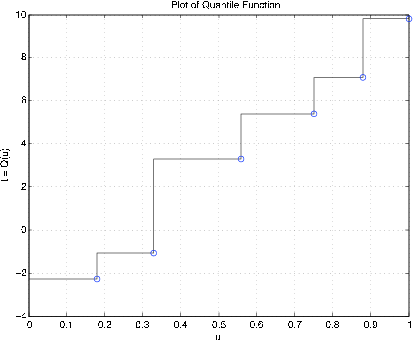
The basis for quantile function calculations for a simple random variable is the formula above. This is implemented in the m-function dquant , which is used as an element of several simulation procedures.To plot the quantile function, we use dquanplot which employs the stairs function and plots X vs the distribution function F X . The procedure dsample employs dquant to obtain a “sample” from a population with simple distribution and tocalculate relative frequencies of the various values.

Simple random variable

X = [-2.3 -1.1 3.3 5.4 7.1 9.8];PX = 0.01*[18 15 23 19 13 12];dquanplot Enter VALUES for X XEnter PROBABILITIES for X PX % See [link] for plot of results rand('seed',0) % Reset random number generator for referencedsample Enter row matrix of values XEnter row matrix of probabilities PX Sample size n 10000 Value Prob Rel freq -2.3000 0.1800 0.1805-1.1000 0.1500 0.1466 3.3000 0.2300 0.23205.4000 0.1900 0.1875 7.1000 0.1300 0.13339.8000 0.1200 0.1201 Sample average ex = 3.325Population mean E[X] = 3.305Sample variance = 16.32 Population variance Var[X]= 16.33
Figure three is a plot of a quantile function on a square gridded graph. The plot looks like a set of stairs, moving from the bottom-left to the top-right of the figure. The vertical axis is t = Q(u), and the horizontal axis is u. the graph begins just below -2 on the vertical axis, and moves horizontally to just before 0.2, where the plot continues after a small blue circle at the vertex with a vertical line extending upward to approximately -1. At this point, the plot then moves right, horizontally, to approximately u=0.33. There is another small blue circle at this vertex, and then the plot continues vertically for a longer segment to approximately 3.5. The plot continues horizontally to the right after this point to approximately u=0.57. At this point, there is a third small blue circle marking the vertex, and then the plot continues vertically upward to approximately 5.5. The plot continues horizontally to the right after this point to approximately u=0.75 where it is met with a fourth small blue circle. The plot moves upward after this point to 7, and then moves to the right to u=0.88. One more vertical segment follows after another small blue circle nearly to 10, where it finally moves to the right to u=1 and is met with a sixth blue circle. Figure three is a plot of a quantile function on a square gridded graph. The plot looks like a set of stairs, moving from the bottom-left to the top-right of the figure. The vertical axis is t = Q(u), and the horizontal axis is u. the graph begins just below -2 on the vertical axis, and moves horizontally to just before 0.2, where the plot continues after a small blue circle at the vertex with a vertical line extending upward to approximately -1. At this point, the plot then moves right, horizontally, to approximately u=0.33. There is another small blue circle at this vertex, and then the plot continues vertically for a longer segment to approximately 3.5. The plot continues horizontally to the right after this point to approximately u=0.57. At this point, there is a third small blue circle marking the vertex, and then the plot continues vertically upward to approximately 5.5. The plot continues horizontally to the right after this point to approximately u=0.75 where it is met with a fourth small blue circle. The plot moves upward after this point to 7, and then moves to the right to u=0.88. One more vertical segment follows after another small blue circle nearly to 10, where it finally moves to the right to u=1 and is met with a sixth blue circle.
Quantile function for [link] .
Got questions? Get instant answers now!

Sometimes it is desirable to know how many trials are required to reach a certain value, or one of a set of values. A pair of m-procedures are available for simulation of that problem.The first is called targetset . It calls for the population distribution and then for the designation of a “target set” of possible values. The second procedure, targetrun , calls for the number of repetitions of the experiment, and asks for the number of members ofthe target set to be reached. After the runs are made, various statistics on the runs are calculated and displayed.

X = [-1.3 0.2 3.7 5.5 7.3]; % Population valuesPX = [0.2 0.1 0.3 0.3 0.1]; % Population probabilitiesE = [-1.3 3.7]; % Set of target statestargetset Enter population VALUES XEnter population PROBABILITIES PX The set of population values is-1.3000 0.2000 3.7000 5.5000 7.3000 Enter the set of target values ECall for targetrun rand('seed',0) % Seed set for possible comparison targetrunEnter the number of repetitions 1000 The target set is-1.3000 3.7000 Enter the number of target values to visit 2The average completion time is 6.32 The standard deviation is 4.089The minimum completion time is 2 The maximum completion time is 30To view a detailed count, call for D. The first column shows the various completion times;the second column shows the numbers of trials yielding those times % Figure 10.6.4 shows the fraction of runs requiring t steps or less
Got questions? Get instant answers now!
Figure four is a fraction of Runs t steps or less. The horizontal axis is t, which is the number of steps to complete the run, and the vertical axis is the fraction of runs. The plot begins from the bottom left with a strong positive slope, and as it moves to the right, the slope becomes more shallow until, at a value of 1 on the horizontal axis, the plot is nearly horizontal, where it terminates exactly at the top-right point on the graph. Figure four is a fraction of Runs t steps or less. The horizontal axis is t, which is the number of steps to complete the run, and the vertical axis is the fraction of runs. The plot begins from the bottom left with a strong positive slope, and as it moves to the right, the slope becomes more shallow until, at a value of 1 on the horizontal axis, the plot is nearly horizontal, where it terminates exactly at the top-right point on the graph.
Fraction of runs requiring t steps or less.

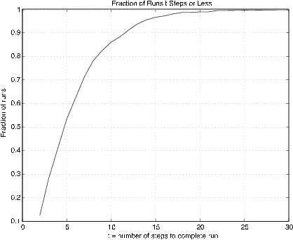
m-procedures for distribution functions

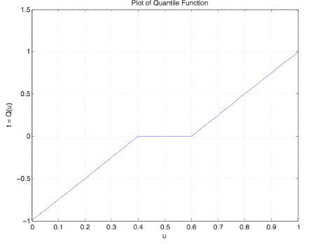
A procedure dfsetup utilizes the distribution function to set up an approximate simple distribution. The m-procedure quanplot is used to plot the quantile function. This procedure is essentially the same as dquanplot, exceptthe ordinary plot function is used in the continuous case whereas the plotting function stairs is used in the discrete case. The m-procedure qsample is used to obtain a sample from the population. Since there are so many possible values, these arenot displayed as in the discrete case.

Quantile function associated with a distribution function.

F = '0.4*(t + 1).*(t<0) + (0.6 + 0.4*t).*(t>= 0)'; % String dfsetupDistribution function F is entered as a string variable, either defined previously or upon callEnter matrix [a b] of X-range endpoints [-1 1]Enter number of X approximation points 1000 Enter distribution function F as function of t FDistribution is in row matrices X and PX quanplotEnter row matrix of values X Enter row matrix of probabilities PXProbability increment h 0.01 % See [link] for plot qsampleEnter row matrix of X values X Enter row matrix of X probabilities PXSample size n 1000 Sample average ex = -0.004146Approximate population mean E(X) = -0.0004002 % Theoretical = 0 Sample variance vx = 0.25Approximate population variance V(X) = 0.2664
Figure five is a plot of the quantile function for example 7. The horizontal axis is labeled u, and the vertical axis is t = Q(u). The plot on the graph begins at the bottom right corner, with the vertical value of -1 and the horizontal value of 0. The plot has a constant positive slope to (0.4, 0), where it extends horizontally to (0.6, 0). Then, the plot continues with the same positive slope as the first segment, where it terminates at (1, 1). Figure five is a plot of the quantile function for example 7. The horizontal axis is labeled u, and the vertical axis is t = Q(u). The plot on the graph begins at the bottom right corner, with the vertical value of -1 and the horizontal value of 0. The plot has a constant positive slope to (0.4, 0), where it extends horizontally to (0.6, 0). Then, the plot continues with the same positive slope as the first segment, where it terminates at (1, 1).
Quantile function for [link] .
Got questions? Get instant answers now!

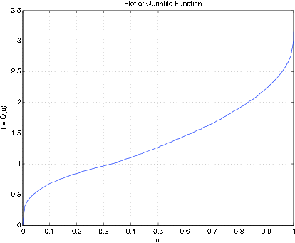
m-procedures for density functions

An m- procedure acsetup is used to obtain the simple approximate distribution. This is essentially the same as the procedure tuappr, except thatthe density function is entered as a string variable. Then the procedures quanplot and qsample are used as in the case of distribution functions.

Quantile function associated with a density function.

acsetup Density f is entered as a string variable.either defined previously or upon call. Enter matrix [a b]of x-range endpoints [0 3] Enter number of x approximation points 1000Enter density as a function of t '(t.^2).*(t<1) + (1- t/3).*(1<=t)' Distribution is in row matrices X and PXquanplot Enter row matrix of values XEnter row matrix of probabilities PX Probability increment h 0.01 % See [link] for plot rand('seed',0)qsample Enter row matrix of values XEnter row matrix of probabilities PX Sample size n 1000Sample average ex = 1.352 Approximate population mean E(X) = 1.361 % Theoretical = 49/36 = 1.3622Sample variance vx = 0.3242 Approximate population variance V(X) = 0.3474 % Theoretical = 0.3474
Figure six is a plot of the quantile function for example 8. The horizontal axis is labeled u, and the vertical axis is t = Q(u). The plot on the graph begins at the bottom-right at (0, 0) with a very steep positive slope. The plot's slope quickly decreases to a shallow positive slope. The plot increases  across the graph, and about halfway across the page the slope begins to progressively increase in the same form that it was previously decreasing, until it terminates at (1, 3) at a very strong (nearly vertical) positive slope. Figure six is a plot of the quantile function for example 8. The horizontal axis is labeled u, and the vertical axis is t = Q(u). The plot on the graph begins at the bottom-right at (0, 0) with a very steep positive slope. The plot's slope quickly decreases to a shallow positive slope. The plot increases  across the graph, and about halfway across the page the slope begins to progressively increase in the same form that it was previously decreasing, until it terminates at (1, 3) at a very strong (nearly vertical) positive slope.
Quantile function for [link] .
Got questions? Get instant answers now!

Get Jobilize Job Search Mobile App in your pocket Now!

Get it on Google Play Download on the App Store Now


Source:  OpenStax, Applied probability. OpenStax CNX. Aug 31, 2009 Download for free at http://cnx.org/content/col10708/1.6
Google Play and the Google Play logo are trademarks of Google Inc.

Notification Switch

Would you like to follow the 'Applied probability' conversation and receive update notifications?

Ask