

| << Chapter < Page | Chapter >> Page > |
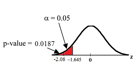
Historical Note: The traditional way to compare the two probabilities, and the p-value, is to compare the critical value (z-score from ) to the test statistic (z-score from data). The calculated test statistic for the p-value is . (From the Central Limit Theorem, the test statistic formula is . For this problem, , from the null hypothesis, , and .) You canfind the critical value for in the normal table (see 15.Tables in the Table of Contents). The z-score for an area to the left equal to 0.05 is midway between -1.65 and -1.64 (0.05 is midway between 0.0505 and 0.0495). The z-score is -1.645.Since (which demonstrates that ), reject . Traditionally, the decision to reject or not reject was done in this way. Today, comparing the two probabilities and the p-value is very common. For this problem, the p-value, is considerably smaller than , 0.05. You can be confident about your decision to reject. The graph shows , the p-value, and the test statistics and the critical value.
A college football coach thought that his players could bench press a mean weight of 275 pounds . It is known that the standard deviation is 55 pounds . Three of his players thought that the mean weight was more than that amount. They asked 30 of their teammates for their estimated maximum lift on the bench press exercise. The data ranged from 205 pounds to 385 pounds. The actualdifferent weights were (frequencies are in parentheses)
Conduct a hypothesis test using a 2.5% level of significance to determine if the bench press mean is more than 275 pounds .
Set up the Hypothesis Test:
Since the problem is about a mean weight, this is a test of a single population mean .
: : This is a right-tailed test.
Calculating the distribution needed:
Random variable: = the mean weight, in pounds, lifted by the football players.
Distribution for the test: It is normal because is known.
~
pounds (from the data).
pounds (Always use if you know it.) We assume pounds unless our data shows us otherwise.
Calculate the p-value using the normal distribution for a mean and using the sample mean as input (see the calculator instructions below for using the data as input):
) .
Interpretation of the p-value: If is true, then there is a 0.1331 probability (13.23%) that the football players can lift a mean weight of 286.2pounds or more. Because a 13.23% chance is large enough, a mean weight lift of 286.2 pounds or more is not a rare event.
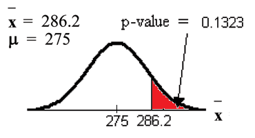
Compare and the p-value:
Make a decision: Since , do not reject .
Conclusion: At the 2.5% level of significance, from the sample data, there is not sufficient evidence to conclude that the true mean weight lifted is more than 275pounds.
The p-value can easily be calculated using the TI-83+ and the TI-84 calculators:
Put the data and frequencies into lists. Press
STAT and arrow over to
TESTS . Press
1:Z-Test . Arrow over to
Data and
press
ENTER . Arrow down and enter 275 for
, 55 for
, the name of the
list where you put the data, and the name of the list where you put thefrequencies. Arrow down to
and arrow over to
. Press
ENTER .
Arrow down to
Calculate and press
ENTER . The calculator not only
calculates the p-value (
, a little different from the above
calculation - in it we used the sample mean rounded to one decimal placeinstead of the data) but it also calculates the test statistic (z-score) for the
sample mean, the sample mean, and the sample standard deviation.
is the alternate hypothesis. Do this set of instructions again except arrow
to
Draw (instead of
Calculate ). Press
ENTER . A shaded graph appears with
(test statistic) and
(p-value). Make sure when you
use
Draw that no other equations are highlighted in
and the plots are
turned off.
Notification Switch
Would you like to follow the 'Elementary statistics' conversation and receive update notifications?

|
|

|
|

|
|

|
|
|
|
|

|
|
|
|
|

|
|

|
|

|