

| << Chapter < Page | Chapter >> Page > |
% file jdemo3.m
% data for joint simple distributionX = [-4 -2 0 1 3];Y = [0 1 2 4];P = [0.0132    0.0198    0.0297    0.0209    0.0264;
     0.0372    0.0558    0.0837    0.0589    0.0744;0.0516    0.0774    0.1161    0.0817    0.1032;
     0.0180    0.0270    0.0405    0.0285    0.0360];
jdemo3                % Call for datajcalc                 % Set up of calculating matrices t, u.
Enter JOINT PROBABILITIES (as on the plane)  PEnter row matrix of VALUES of X  X
Enter row matrix of VALUES of Y  YUse array operations on matrices X, Y, PX, PY, t, u, and P
G = t.^2 -3*u;        % Formation of G = [g(ti,uj)]M = G>= 1;           % Calculation using the XY distribution
PM = total(M.*P)      % Alternately, use total((G>=1).*P)
PM =  0.4665[Z,PZ] = csort(G,P);PM = (Z>=1)*PZ'     % Calculation using the Z distribution
PM =  0.4665disp([Z;PZ]')         % Display of the Z distribution-12.0000    0.0297
  -11.0000    0.0209-8.0000    0.0198
   -6.0000    0.0837-5.0000    0.0589
   -3.0000    0.1425-2.0000    0.1375
         0    0.04051.0000    0.1059
    3.0000    0.07444.0000    0.0402
    6.0000    0.10329.0000    0.0360
   10.0000    0.037213.0000    0.0516
16.0000 0.0180 We extend the example above by considering a function which has a composite definition.
Let
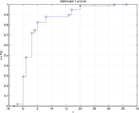
H = t.*(t+u>=1) + (t.^2 + u.^2).*(t+u<1);  % Specification of h(t,u)[W,PW] = csort(H,P);                       % Distribution for W = h(X,Y)disp([W;PW]')-2.0000    0.0198
         0    0.27001.0000    0.1900
    3.0000    0.24004.0000    0.0270
    5.0000    0.07748.0000    0.0558
   16.0000    0.018017.0000    0.0516
   20.0000    0.037232.0000    0.0132
ddbn                                        % Plot of distribution functionEnter row matrix of values  W
Enter row matrix of probabilities  PWprint                                       % See
[link]
Joint distributions for two functions of
In previous treatments, we use csort to obtain the marginal distribution for a single function . It is often desirable to have the joint distribution for a pair and . As special cases, we may have or . Suppose
The joint distribution requires the probability of each pair, . Each such pair of values corresponds to a set of pairs of X and Y values. To determine the joint probability matrix for arranged as on the plane, we assign to each position the probability , with values of W increasing upward. Each pair of values corresponds to one or more pairs of values. If we select and add the probabilities corresponding to the latter pairs, we have . This may be accomplished as follows:
Notification Switch
Would you like to follow the 'Applied probability' conversation and receive update notifications?

|
|

|
|

|
|

|
|

|
|

|
|

|
|

|
|

|
|

|