For a pair {X, Y} having joint distribution on the plane, the approach is analogous to the single variable case. To find the probability an absolutely continuous pair takes on values in a set Q on the plane, integrate the joint density over the set. In the discrete case, identify those pairs of values which meet the defining conditions for Q and add the associated probabilities. To find the probability that g(X, Y ) takes on a a value in set M, determine the set Q of those pairs (t, u) mapped into M by the function g and then determine, as in the previous case, the probability the pair {X, Y} takes on values in Q.
Introduction
The general mapping approach for a single random variable and the discrete alternative
extends to functions of more than one variable. It is convenient to consider thecase of two random variables, considered jointly. Extensions
to more than two random variables are made similarly, although the details are more complicated.
The general approach extended to a pair
Consider a pair
having joint distribution on the plane. The approach is analogous
to that for a single random variable with distribution on the line.
To find
.
Mapping approach . Simply find the amount of probability mass mapped into
the set
Q on the plane by the random vector
.
In the absolutely continuous case, calculate
.
In the discrete case, identify those vector values
of
which are
in the set
Q and add the associated probabilities.
Discrete alternative . Consider each vector value
of
. Select those which meet the defining conditions for
Q and add the associated probabilities. This
is the approach we use in the MATLAB calculations. It does not require that we describe geometricallythe region
Q .
To find
.
g is real valued and
M is a subset the real line.
Mapping approach . Determine the set
Q of all those
which are
mapped into
M by the function
g . Now
Since these are the same event, they must have the same probability. Once
Q is identified
on the plane,determine
in the usual manner (see part a, above).
Discrete alternative . For each possible vector value
of
, determine whether
meets the defining condition for
M . Select
those
which do and add the associated probabilities.
We illustrate the mapping approach in the absolutely continuous case. A key element in the
approach is finding the set
Q on the plane such that
iff
. The desired probability is obtained by integrating
over
Q .
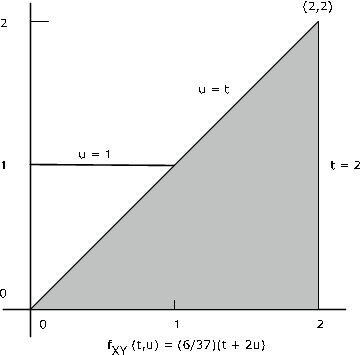
The pair
has joint density
on the region bounded by
,
,
,
(see Figure 1).
Determine
. Here
and
. Now
which is the region on the
plane on or below the line
. Examination of the figure shows that for this region,
is different from zero on the triangle bounded by
,
, and
.
The desired probability is