1.4 Quantizer design for entropy coded sytems

An introduction to source-coding Page 1 / 1

Motivated by the cascade of memoryless quantization and entropy coding, the entropy-minimizing scalar memoryless quantizer is derived. Using a compander formulation and tools from the calculus of variations, it is shown that the entropy-minimizing quantizer is the simple uniform quantizer. The penalty associated with memoryless quantization is then analyzed in the asymptotic case of many quantization levels.

Say that we are designing a system with a memoryless quantizer followed by an entropy coder, and our goal is to minimize theaverage transmission rate for a given σ _q ² (or vice versa). Is it optimal to cascade a σ _q ² -minimizing (Lloyd-Max) quantizer with a rate-minimizing code?In other words, what is the optimal memoryless quantizer if the quantized outputs are to be entropy coded?
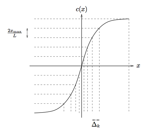
A Compander Formulation: To determine the optimal quantizer,
1. consider a companding system: a memoryless nonlinearity $c (x)$ followed by uniform quantizer,
2. find $c (x)$ minimizing entropy H _y for a fixed error variance σ _q ² .
Compander curve: nonuniform input regions mapped to uniform output regions (for subsequent uniform quantization)
First we must express σ _q ² and H _y in terms of $c (x)$ . [link] suggests that, for large L , the slope $c^{'} (x) : = d c (x) / d x$ obeys
$c^{'} (x) |_{x \in X_{k}} = \frac{2 x_{max} / L}{Δ_{k}},$
so that we may write
$Δ_{k} = \frac{2 x_{max}}{L c^{'} (x)} |_{x \in X_{k}} .$
Assuming large L , the σ _q ² -approximation equation 9 from MSE-Optimal Memoryless Scalar Quantization (lower equation) can be transformed as follows.
$\begin{matrix} σ_{q}^{2} & = & \frac{1}{12} \sum_{k = 1}^{L} P_{k} Δ_{k}^{2} \\ = & \frac{x_{max}^{2}}{3 L^{2}} \sum_{k = 1}^{L} \frac{P_{k}}{c^{'} {(x)}^{2}} |_{x \in X_{k}} \\ = & \frac{x_{max}^{2}}{3 L^{2}} \sum_{k = 1}^{L} \frac{p_{x} (x)}{c^{'} {(x)}^{2}} Δ_{k} |_{x \in X_{k}} since P_{k} = p_{x} (x) |_{x \in X_{k}} Δ_{k} for large L \\ = & \frac{x_{max}^{2}}{3 L^{2}} \int_{- x_{max}}^{x_{max}} \frac{p_{x} (x)}{c^{'} {(x)}^{2}} d x . \end{matrix}$
Similarly,
$\begin{matrix} H_{y} & = & - \sum_{k = 1}^{L} P_{k} {log}_{2} P_{k} \\ = & - \sum_{k = 1}^{L} p_{x} (x) Δ_{k} {log}_{2} (p_{x}, (x), Δ_{k}) |_{x \in X_{k}} \\ = & - \sum_{k = 1}^{L} p_{x} (x) Δ_{k} {log}_{2} p_{x} (x) |_{x \in X_{k}} - \sum_{k = 1}^{L} p_{x} (x) Δ_{k} {log}_{2} Δ_{k} |_{x \in X_{k}} \\ = & \underset{h_{x} : ``differential entropy''}{\underset{︸}{- \int_{- x_{max}}^{x_{max}} p_{x} (x) {log}_{2} p_{x} (x) d x}} - \int_{- x_{max}}^{x_{max}} p_{x} (x) {log}_{2} \underset{Δ_{k}}{\underset{︸}{\frac{2 x_{max}}{L c^{'} (x)}}} d x \\ = & h_{x} - {log}_{2} \frac{2 x_{max}}{L} \underset{= 1}{\underset{︸}{\int_{- x_{max}}^{x_{max}} p_{x} (x) d x}} + \int_{- x_{max}}^{x_{max}} p_{x} (x) {log}_{2} c^{'} (x) d x \\ = & constant + \int_{- x_{max}}^{x_{max}} p_{x} (x) {log}_{2} c^{'} (x) d x \end{matrix}$
Entropy-Minimizing Quantizer: Our goal is to choose $c (x)$ which minimizes the entropy rate H _y subject to fixed error variance σ _q ² . We employ a Lagrange technique again, minimizingthe cost $\int_{- x_{max}}^{x_{max}} p_{x} (x) {log}_{2} c^{'} (x) d x$ under the constraint that the quantity $\int_{- x_{max}}^{x_{max}} p_{x} (x) {(c^{'}, (x))}^{- 2} d x$ equals a constant C . This yields the unconstrained cost function
$\begin{matrix} J_{u} (c^{'} (x), λ) = \int_{- x_{max}}^{x_{max}} \underset{φ (c^{'} (x), λ)}{\underset{︸}{[p_{x} (x) {log}_{2} c^{'} (x) + λ (p_{x} (x) {(c^{'}, (x))}^{- 2} - C)]}} d x, \end{matrix}$
with scalar λ , and the unconstrained optimization problem becomes
$min_{c^{'} (x), λ} J_{u} (c^{'} (x), λ) .$
The following technique is common in variational calculus (see, e.g., Optimal Systems Control by Sage&White). Say $a^{⋆} (x)$ minimizes a (scalar) cost $J (a (x))$ . Then for any (well-behaved) variation $η (x)$ from this optimal $a^{⋆} (x)$ , we must have
$\frac{\partial}{\partial ϵ} J (a^{⋆} (x) + ϵ η (x)) |_{ϵ = 0} = 0$
where ϵ is a scalar. Applying this principle to our optimization problem, we search for $c^{'} (x)$ such that
$\forall η (x), \frac{\partial}{\partial ϵ} J_{u} (c^{'} (x) + ϵ η (x), λ) |_{ϵ = 0} = 0 .$
From [link] we find (using ${log}_{2} a = {log}_{2} e \cdot {log}_{e} a$ )
$\begin{matrix} \frac{\partial J_{u}}{\partial ϵ} |_{ϵ = 0} & = & \int_{- x_{max}}^{x_{max}} \frac{\partial}{\partial ϵ} φ (c^{'} (x) + ϵ η (x), λ) |_{ϵ = 0} d x \\ = & \int_{- x_{max}}^{x_{max}} \frac{\partial}{\partial ϵ} [p_{x} (x) {log}_{2} (e) {log}_{e} (c^{'} (x) + ϵ η (x)) + λ (p_{x} (x) {(c^{'} (x) + ϵ η (x))}^{- 2} - C)] |_{ϵ = 0} d x \\ = & \int_{- x_{max}}^{x_{max}} [{log}_{2} (e) p_{x} (x) {(c^{'} (x) + ϵ η (x))}^{- 1} η (x) - 2 λ p_{x} (x) {(c^{'} (x) + ϵ η (x))}^{- 3} η (x)] |_{ϵ = 0} d x \\ = & \int_{- x_{max}}^{x_{max}} p_{x} (x) {(c^{'}, (x))}^{- 1} [{log}_{2} (e) - 2 λ {(c^{'}, (x))}^{- 2}] η (x) d x \end{matrix}$
and to allow for any $η (x)$ we require
${log}_{2} (e) - 2 λ {(c^{'}, (x))}^{- 2} = 0 \Leftrightarrow c^{'} (x) = \underset{a constant!}{\underset{︸}{\sqrt{\frac{2 λ}{{log}_{2} e}}}} .$
Applying the boundary conditions,
$\{\begin{matrix} c (x_{max}) = x_{max} \\ c (- x_{max}) = - x_{max} \end{matrix}\} \to \begin{matrix} c (x) = x \end{matrix} .$
Thus, for large- L , the quantizer that minimizes entropy rate H _y for a given quantization error variance σ _q ² is the uniform quantizer. Plugging $c (x) = x$ into [link] , the rightmost integral disappears and we have
$H_{y} |_{uniform} = h_{x} - {log}_{2} \underset{Δ}{\underset{︸}{\frac{2 x_{max}}{L}}},$
and using the large- L uniform quantizer error variance approximation equation 6 from Memoryless Scalar Quantization ,
$H_{y} |_{uniform} = h_{x} - \frac{1}{2} {log}_{2} (12, σ_{q}^{2}) .$
It is interesting to compare this result to the information-theoretic minimal average rate for transmission of a continuous-amplitudememoryless source x of differential entropy h _x at average distortion σ _q ² (see Jayant&Noll or Berger):
$R_{min} = h_{x} - \frac{1}{2} {log}_{2} (2, π, e, σ_{q}^{2}) .$
Comparing the previous two equations, we find that (for a continous-amplitude memoryless source) uniform quantizationprior to entropy coding requires
$\frac{1}{2} {log}_{2} (\frac{π e}{6}) \approx \begin{matrix} 0.255 bits/sample \end{matrix}$
more than the theoretically optimum transmission scheme, regardless of the distribution of x . Thus, 0.255 bits/sample (or $\sim 1.5$ dB using the $6.02 R$ relationship) is the price paid for memoryless quantization .

<< Chapter < Page Page > Chapter >>

Read also:

Get Jobilize Job Search Mobile App in your pocket Now!

100% Free Mobile Applications
Receive real-time job alerts and never miss the right job again

Source: OpenStax, An introduction to source-coding: quantization, dpcm, transform coding, and sub-band coding. OpenStax CNX. Sep 25, 2009 Download for free at http://cnx.org/content/col11121/1.2

Google Play and the Google Play logo are trademarks of Google Inc.

Notification Switch

Would you like to follow the 'An introduction to source-coding: quantization, dpcm, transform coding, and sub-band coding' conversation and receive update notifications?

Ask

	MAPEH Test G9 (Physical Education) By Angelica Lito Start Quiz
	22 AP 22 Respiratory System MCQ By OpenStax Start Quiz
	9 Biology 09 Cell Communication MCQ By OpenStax Start Quiz
	Social Dances 1 By Marion Cabalfin Start Test
	How much do you love him? By Zarina Chocolate Start Quiz
	20 AP 20 Blood Vessels Circulation Essay By OpenStax Start Flashcards
	12 Dr Dowers Endocrinology By Brooke Delaney Start Exam
	20 AP 20 Blood Vessels Circulation MCQ By OpenStax Start Quiz
	24 AP 24 Metabolism Nutrition MCQ By OpenStax Start Quiz
	1 Understanding Societies 1 By Jessica Collett Start Exam