1.3 Optimal encoding of bandlimited signals

We now turn back to the encoding of signals. We are interested in encoding the set

We shall sketch how one can construct an asymptotically optimal encoder/decoder for $B_A$ . The details for this construction can be found in [link] .

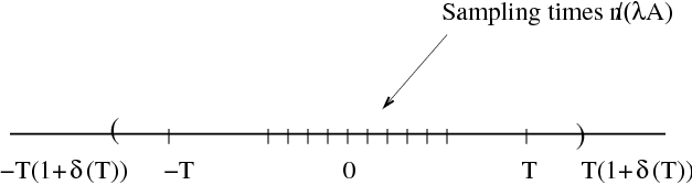
We know $\widehat{f}\left(\omega \right)=0$ for $\left|\omega \right|\ge A\pi$ , and $\left|f\right|\le M$ . How can we encode $f$ in practice? We begin by chosing $\lambda =\lambda \left(T\right)>1$ (see [link] ) which will represent a slight oversampling factor we shall utilize.Given a target distortion $ϵ>0$ , we choose $k$ so that $2^{-k-1}<ϵ\le 2^{-k}$ . Given $f$ , we shall encode $f$ by first taking samples $f\left(\frac{n}{\lambda A}\right)$ for $\frac{n}{\lambda A}\in [-T(1+\delta ),T(1+\delta \left)\right]$ where $\delta \left(T\right)>0$ . In other words, we sample $f$ on a slightly larger interval than $[-T,T]$ . For each sample $f\left(\frac{n}{\lambda A}\right)$ , we shall use the first $k+k_0\left(T\right)$ bits of its binary expansion. In other words, our encoder takes $f$ and the samples $f\left(\frac{n}{\lambda A}\right)$ and then assigns to $f\left(\frac{n}{\lambda A}\right)$ the first $k+k_0\left(T\right)$ bits of this number.

To decode, the receiver would take the bits and construct the approximation $\overline{f}(\frac{n}{\lambda A})$ to $f\left(\frac{n}{A\lambda }\right)$ from the bits provided. Notice that we have the accuracy

The term $\left|f,\left(\frac{n}{\lambda A}\right),-,\overline{f},\left(\frac{n}{\lambda A}\right)\right|$ that appears in the first summation in ( [link] ) is bounded by $M·2^{-k-k_0}$ . The term $\left|f,\left(\frac{n}{\lambda A}\right)\right|$ that appears in the second summation in the same equation is bounded by $M$ . Therefore,

To make the encoder/decoder specific we need to precisely define $\delta$ and $\lambda$ . It turns out that the best choices (in terms of bit rate performance on the class $B_A$ ) depend on $T$ . But ${\delta }_T\to 0$ and ${\lambda }_T\to 1$ as $T\to \infty$ . Recall that Shannon sampling requires $2T\lambda A$ samples. Since our encoder/decoder uses $k+k_0$ bits per sample, the total number of bits is $(k+k_0)·2\lambda AT(1+\delta )$ , and so coding will require roughly $k$ bits per Shannon sample.

This encoder/decoder can be proven to be optimal in the sense of averaged performance as we shall now describe. The average of performance of optimal encoding is defined by

In summary, to encode band limited signals on an interval $[-T,T]$ , an optimal strategy is to sample at a slightly higher rate than Nyquist and on a slightly large interval than $[-T,T]$ . Each sample should then be quantized by using the binary expansion of the sample. In this way, for an investment of $k$ bits per Nyquist rate sample, we get a distortion of $2^{-k}$ .

To get a feel for the number of bits required by such an encoder, let us say $A={10}^6$ (signals band limited to 1Mhz). Say $T=24\text{hours}\approx {10}^5\text{seconds}$ , and $k=10$ bits. Then, $A·k·2T={10}^6·10·{10}^5={10}^{12}$ bits. This is too BIG!

The above encoding is is known as Pulse Coded Modulation (PCM). In practice,people frequently use another encoder called Sigma-Delta Modulation. Instead of oversampling just slightly, Sigma Delta over samples a lot and then assign only one (or a few) bits per sample.

Why is Sigma-Delta preferred to PCM in practice? There are two reasons commonly given:

1. Getting accurate samples, quantization, etc. is not practical because of noise. For better accuracy, we need moreexpensive hardware.
2. Noise shaping. In Sigma-Delta, the distortion is higher but the distortion is spread over frequencies outside of the desiredrange.

In PCM, the distortion decays exponentially (like $2^{-k}$ ), whereas for Sigma-Delta, the distortion decays like a polynomial (like $\frac{1}{k^m}$ ). Although the distortion decays faster in PCM, the distortion in Sigma-Delta is spread outside the desired frequencyrange.