

| << Chapter < Page | Chapter >> Page > |
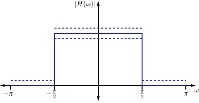
So far, our approximation problem has been posed in an inner product space, and we have thus measured our approximation error using norms that are induced by an inner product such as the norms (or weighted norms). Sometimes this is a natural choice – it can be interpreted as the “energy” in the error and arises often in the case of signals corrupted by Gaussian noise. However, more often than not, it is used simply because it is easy to deal with.
In some cases we might be interested in approximating with respect to other norms – in particular we will consider approximation with respect to -norms for . First, we introduce the concept of a “unit ball”. Any norm gives us rise to a unit ball, i.e., Some important examples of unit balls for the norms in are depicted below.


We now consider an example of approximating a point in with a point in a 1-D subspace while measuring error using the norm for .
Suppose ,
We will want to find that minimizes . Since , we can write
and thus
While we can solve for to minimize directly in some cases, a geometric interpretation is also useful. In each case, on can imagine growing an ball centered on until the ball intersects with . This will be the point . that is closest to in the norm. We first illustrate this for the norm below:

In order to calculate we can apply the orthogonality principle. Since we obtain a solution defined by .
We now observe that in the case of the norm the picture changes somewhat. The closest point in is illustrated below:
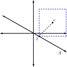
Note that the error is no longer orthogonal to the subspace . In this case we can still calculate from the observation that the two terms in the error should be equal, which yields .
The situation is even more different for the case of the norm, which is illustrated below:

We now observe that corresponds to . Note that in this case the error term is . This punctuates a general trend: for large values of , the norm tends to spread error evenly across all terms, while for small values of the error is more highly concentrated.
When is it useful to approximate in or norms for ?
Notification Switch
Would you like to follow the 'Digital signal processing' conversation and receive update notifications?

|
|

|
|

|
|

|
|

|
|
|
|
|

|
|

|
|

|
|

|