1.2 Calculus of parametric curves (Page 3/6)

Calculus volume 3 Page 3 / 6

Then a Riemann sum for the area is

A_{n} = \sum_{i = 1}^{n} y (x ({\bar{t}}_{i})) (x (t_{i}) - x (t_{i - 1})) .

Multiplying and dividing each area by $t_{i} - t_{i - 1}$ gives

A_{n} = \sum_{i = 1}^{n} y (x ({\bar{t}}_{i})) (\frac{x (t_{i}) - x (t_{i - 1})}{t_{i} - t_{i - 1}}) (t_{i} - t_{i - 1}) = \sum_{i = 1}^{n} y (x ({\bar{t}}_{i})) (\frac{x (t_{i}) - x (t_{i - 1})}{Δ t}) Δ t .

Taking the limit as $n$ approaches infinity gives

A = lim_{n \to \infty} A_{n} = \int_{a}^{b} y (t) x^{'} (t) d t .

This leads to the following theorem.

Area under a parametric curve

Consider the non-self-intersecting plane curve defined by the parametric equations

x = x (t), y = y (t), a \leq t \leq b

and assume that $x (t)$ is differentiable. The area under this curve is given by

A = \int_{a}^{b} y (t) x^{'} (t) d t .

Finding the area under a parametric curve

Find the area under the curve of the cycloid defined by the equations

x (t) = t - sin t, y (t) = 1 - cos t, 0 \leq t \leq 2 π .

Using [link] , we have

\begin{matrix} A & = \int_{a}^{b} y (t) x^{'} (t) d t \\ = \int_{0}^{2 π} (1 - cos t) (1 - cos t) d t \\ = \int_{0}^{2 π} (1 - 2 cos t + {cos}^{2} t) d t \\ = \int_{0}^{2 π} (1 - 2 cos t + \frac{1 + cos 2 t}{2}) d t \\ = \int_{0}^{2 π} (\frac{3}{2} - 2 cos t + \frac{cos 2 t}{2}) d t \\ = {\frac{3 t}{2} - 2 sin t + \frac{sin 2 t}{4} |}_{0}^{2 π} \\ = 3 π . \end{matrix}

Got questions? Get instant answers now!

Find the area under the curve of the hypocycloid defined by the equations

x (t) = 3 cos t + cos 3 t, y (t) = 3 sin t - sin 3 t, 0 \leq t \leq π .

$A = 3 π$ (Note that the integral formula actually yields a negative answer. This is due to the fact that $x (t)$ is a decreasing function over the interval $[0, 2 π];$ that is, the curve is traced from right to left.)

Got questions? Get instant answers now!

Arc length of a parametric curve

In addition to finding the area under a parametric curve, we sometimes need to find the arc length of a parametric curve. In the case of a line segment, arc length is the same as the distance between the endpoints. If a particle travels from point A to point B along a curve, then the distance that particle travels is the arc length. To develop a formula for arc length, we start with an approximation by line segments as shown in the following graph.

A curved line in the first quadrant with points marked for x = 1, 2, 3, 4, and 5. These points have values roughly 2.1, 2.7, 3, 2.7, and 2.1, respectively. The points for x = 1 and 5 are marked A and B, respectively. — Approximation of a curve by line segments.

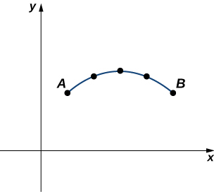
Given a plane curve defined by the functions $x = x (t), y = y (t), a \leq t \leq b,$ we start by partitioning the interval $[a, b]$ into n equal subintervals: $t_{0} = a < t_{1} < t_{2} < ⋯ < t_{n} = b .$ The width of each subinterval is given by $Δ t = (b - a) / n .$ We can calculate the length of each line segment:

\begin{matrix} d_{1} = \sqrt{{(x (t_{1}) - x (t_{0}))}^{2} + {(y (t_{1}) - y (t_{0}))}^{2}} \\ d_{2} = \sqrt{{(x (t_{2}) - x (t_{1}))}^{2} + {(y (t_{2}) - y (t_{1}))}^{2}} etc . \end{matrix}

Then add these up. We let s denote the exact arc length and $s_{n}$ denote the approximation by n line segments:

s \approx \sum_{k = 1}^{n} s_{k} = \sum_{k = 1}^{n} \sqrt{{(x (t_{k}) - x (t_{k - 1}))}^{2} + {(y (t_{k}) - y (t_{k - 1}))}^{2}} .

If we assume that $x (t)$ and $y (t)$ are differentiable functions of t, then the Mean Value Theorem ( Introduction to the Applications of Derivatives ) applies, so in each subinterval $[t_{k - 1}, t_{k}]$ there exist ${\hat{t}}_{k}$ and ${\tilde{t}}_{k}$ such that

\begin{matrix} x (t_{k}) - x (t_{k - 1}) = x^{'} ({\hat{t}}_{k}) (t_{k} - t_{k - 1}) = x^{'} ({\hat{t}}_{k}) Δ t \\ y (t_{k}) - y (t_{k - 1}) = y^{'} ({\tilde{t}}_{k}) (t_{k} - t_{k - 1}) = y^{'} ({\tilde{t}}_{k}) Δ t . \end{matrix}

Therefore [link] becomes

\begin{matrix} s & \approx \sum_{k = 1}^{n} s_{k} \\ = \sum_{k = 1}^{n} \sqrt{{(x^{'} ({\hat{t}}_{k}) Δ t)}^{2} + {(y^{'} ({\tilde{t}}_{k}) Δ t)}^{2}} \\ = \sum_{k = 1}^{n} \sqrt{{(x^{'} ({\hat{t}}_{k}))}^{2} {(Δ t)}^{2} + {(y^{'} ({\tilde{t}}_{k}))}^{2} {(Δ t)}^{2}} \\ = (\sum_{k = 1}^{n} \sqrt{{(x^{'} ({\hat{t}}_{k}))}^{2} + {(y^{'} ({\tilde{t}}_{k}))}^{2}}) Δ t . \end{matrix}

This is a Riemann sum that approximates the arc length over a partition of the interval $[a, b] .$ If we further assume that the derivatives are continuous and let the number of points in the partition increase without bound, the approximation approaches the exact arc length. This gives

\begin{matrix} s & = lim_{n \to \infty} \sum_{k = 1}^{n} s_{k} \\ = lim_{n \to \infty} (\sum_{k = 1}^{n} \sqrt{{(x^{'} ({\hat{t}}_{k}))}^{2} + {(y^{'} ({\tilde{t}}_{k}))}^{2}}) Δ t \\ = \int_{a}^{b} \sqrt{{(x^{'} (t))}^{2} + {(y^{'} (t))}^{2}} d t . \end{matrix}

When taking the limit, the values of ${\hat{t}}_{k}$ and ${\tilde{t}}_{k}$ are both contained within the same ever-shrinking interval of width $Δ t,$ so they must converge to the same value.

<< Chapter < Page Page > Chapter >>

Read also:

Get Jobilize Job Search Mobile App in your pocket Now!

100% Free Mobile Applications
Receive real-time job alerts and never miss the right job again

Source: OpenStax, Calculus volume 3. OpenStax CNX. Feb 05, 2016 Download for free at http://legacy.cnx.org/content/col11966/1.2

Google Play and the Google Play logo are trademarks of Google Inc.

Notification Switch

Would you like to follow the 'Calculus volume 3' conversation and receive update notifications?

Ask

	Spreadsheets MCQ By Ryan Lowe Start Quiz
	Macroeconomics By OpenStax Read Online Course
	4 Psychology MCQ 2009 Final Exam By John Gabrieli Start Exam
	26 AP 26 Fluid, Electrolyte, Acid-Base Balance MCQ By OpenStax Start Quiz
	1 Neuroscience Exam 2004 1 By David Corey Start Exam
	Foundations of Software Engineering By Kevin Amaratunga Start Quiz
	22 AP 22 Respiratory System MCQ By OpenStax Start Quiz
	Does your crush like you? By Hoy Wen Start Quiz
	8 AP 08 Appendicular Skeleton MCQ By OpenStax Start Quiz
	10 Physiotherapy Modalities-Thermo By Rhodes Start Quiz