<< Chapter < Page Chapter >> Page >
- P = ρ g cos β = ρ g sin α , α = π / 2 - β

The equations of motion are as follows.

0 = d P d x 0 = ρ g cos β - d τ x z d x 0 = ρ g cos β + μ d 2 v z d x 2 , Newtonian fluid

The boundary conditions are zero stress at the gas-liquid interface and no slip at the wall.

v z = 0 , x = 0 τ x z = 0 , x = h

The shear stress profile can be determined by integration and application of the zero stress boundary condition.

τ x z = ρ g h cos β x h - 1 , 0 x h τ w = - ρ g h cos β

The velocity profile for a Newtonian fluid can be determined by a second integration and application of the no slip boundary condition.

v z = ρ g h 2 cos β 2 μ 2 x h - x h 2 , 0 x h v z , max = ρ g h 2 cos β 2 μ

The average velocity and volumetric flow rate can be determined by integration of the velocity profile over the film thickness.

v z = ρ g h 2 cos β 3 μ Q = ρ g W h 3 cos β 3 μ

The film thickness, h, can be given in terms of the average velocity, the volume rate of flow, or the mass rate of flow per unit width of wall ( Γ = ρ h v z ) :

h = 3 μ v z ρ g cos β = 3 μ Q ρ g W cos β 3 = 3 μ Γ ρ 2 g cos β 3

Unsteady viscous flow

Suddenly accelerated plate. (BSL, 1960) A semi-infinite body of liquid with constant density and viscosity is bounded on one side by a flat surface ( the x z plane). Initially the fluid and solid surface is at rest; but at time t = 0 the solid surface is set in motion in the positive x -direction with a velocity U . It is desired to know the velocity as a function of y and t . The pressure is hydrostatic and the flow is assumed to be laminar.

The only nonzero component of velocity is v x = v x ( y , t ) . Thus the only non-zero equation of motion is as follows.

ρ v x t = μ 2 v x y 2 , y > 0 , t > 0

The initial condition and boundary conditions are as follows.

v x = 0 , t = 0 , y > 0 v x = U , y = 0 , t > 0 v x = 0 , y , t > 0

If we normalize the velocity with respect to the boundary condition, we see that this is the same parabolic PDE and boundary condition as we solved with a similarity transformation. Thus the solution is

v x = U e r f c y 4 μ t / ρ

The presence of the ratio of viscosity and density, the kinematic viscosity, in the expression for the velocity implies that both viscous and inertial forces are operative.

The velocity profiles for the wall at y = 0 suddenly set in motion is illustrated below.

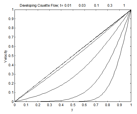
Developing Couette flow. The transient development to the steady-state Couette flow discussed earlier can now be easily derived. We will let the plane y = 0 be the surface with zero velocity and let the velocity be specified at y = L . The initial and boundary conditions are as follows.

v x = 0 , t = 0 , 0 < y < L v x = 0 , y = 0 , t > 0 v x = U , y = L , t > 0 or v x = 0 , t = 0 , - L < y < L v x = - U , y = - L , t > 0 v x = U , y = L , t > 0

It should be apparent that the two formulations of the boundary conditions give the same solution. However, the latter gives a clue how one should obtain a solution. The solution is antisymmetric about y = 0 and the zero velocity condition is satisfied. A series of additional terms are needed to satisfy the boundary conditions at y = ± L . The solution is

v x = U n = 0 e r f c ( 2 n + 1 ) L - y 4 ν t - e r f c ( 2 n + 1 ) L + y 4 ν t ν = μ ρ

Asignment. 8.3

Flow of a fluid with a suddenly applied constant wall stress. This problem is similar to that of flow - < x < , y > 0 , t > 0 near a wall - < x < , y = 0 suddenly set into motion, except that the shear stress at the wall is constant rather than the velocity. Let the fluid be at rest before t = 0 . At time t = 0 a constant force is applied to the fluid at the wall, so that the shear stress τ y x takes on a new constant value τ o at y = 0 for t > 0 .
  1. Start with the continuity and Navier-Stokes equations and eliminate the terms that are identically zero. Differentiate the resulting equation with respect to distance from the wall and multiply by viscosity to derive an equation for the evolution of the shear stress. List all assumptions.
  2. Write the boundary and initial conditions for this equation.
  3. Solve for the time and distance dependence of the shear stress. Sketch the solution.
  4. Calculate the velocity profile from the solution of the shear stress. The following equation will be helpful.
  5. Suppose the fluid is not infinite but rather there is another wall at a distance 2h away from the original wall and it was also set into motion but in the opposite direction with the same wall shear stress. What are the stress and velocity profiles for the fluid between the two walls? Sketch and express as series solutions.
  6. What are the steady state stress and velocity profiles for the problem of part (e)? Sketch and express as analytical solutions.

Get Jobilize Job Search Mobile App in your pocket Now!

Get it on Google Play Download on the App Store Now


Source:  OpenStax, Transport phenomena. OpenStax CNX. May 24, 2010 Download for free at http://cnx.org/content/col11205/1.1
Google Play and the Google Play logo are trademarks of Google Inc.

Notification Switch

Would you like to follow the 'Transport phenomena' conversation and receive update notifications?

Ask