

| << Chapter < Page | Chapter >> Page > |
The second statement of the theorem differs from the first in the following respect: when , there will necessarily exist -sparse signals that cannot be uniquely recovered from the -dimensional measurement vector . However, these signals form a set of measure zero within the set of all -sparse signals and can safely be avoided if is randomly generated independently of .
Unfortunately, as discussed in Nonlinear Approximation from Approximation , solving this optimization problem is prohibitively complex. Yet another challenge is robustness; in the setting ofTheorem "Recovery via ℓ 0 optimization" , the recovery may be very poorly conditioned. In fact, both of these considerations (computational complexity and robustness) can be addressed, but atthe expense of slightly more measurements.
The practical revelation that supports the new CS theory is that it is not necessary to solve the -minimization problem to recover . In fact, a much easier problem yields an equivalent solution (thanks again to the incoherency of thebases); we need only solve for the -sparsest coefficients that agree with the measurements [link] , [link] , [link] , [link] , [link] , [link] , [link] , [link]
There is no free lunch, however; according to the theory, more than measurements are required in order to recover sparse signals via Basis Pursuit. Instead, one typically requires measurements, where is an oversampling factor . As an example, we quote a result asymptotic in . For simplicity, we assume that the sparsity scales linearly with ; that is, , where we call the sparsity rate .
Theorem[link] , [link] , [link] Set with . Then there exists an oversampling factor , , such that, for a -sparse signal in the basis , the following statements hold:
In an illuminating series of recent papers, Donoho and Tanner [link] , [link] , [link] have characterized the oversampling factor precisely (see also "The geometry of Compressed Sensing" ). With appropriate oversampling, reconstruction via Basis Pursuit is also provably robust tomeasurement noise and quantization error [link] .
We often use the abbreviated notation to describe the oversampling factor required in various settings even though depends on the sparsity and signal length .
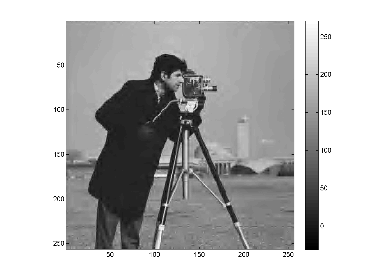
A CS recovery example on the Cameraman test image is shown in [link] . In this case, with we achieve near-perfect recovery of the sparse measured image.
Notification Switch
Would you like to follow the 'Concise signal models' conversation and receive update notifications?

|
|

|
|

|
|

|
|

|
|

|
|

|
|

|
|

|
|

|