

| << Chapter < Page | Chapter >> Page > |
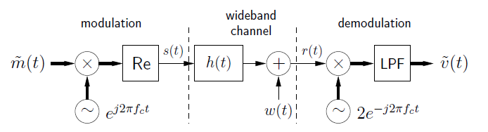
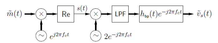
Linear communication schemes (e.g., AM, QAM, VSB) can all be represented (using complex-baseband mod/demod) as:
It turns out that this diagram can be greatly simplified...
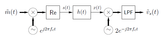
First, consider the signal path on its own:
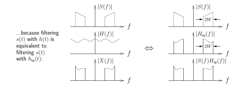
Since is a bandpass signal, we can replace the wideband channel response with its bandpass equivalent :
Then, notice that
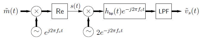
which means we can rewrite the block diagram as
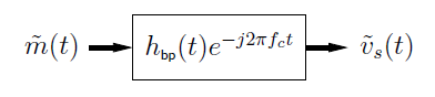
We can now reverse the order of the LPF and (since both are LTI systems), giving
Since mod/demod is transparent (with synched oscillators), it can be removed, simplifying the block diagram to
Now, since is bandlimited to W Hz, there is no need to model the left component of :
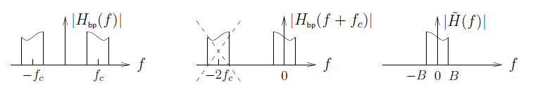
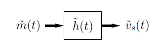
Replacing with the complex-baseband response gives the “complex-baseband equivalent” signal path:
The spectrums above show that .
Next consider the noise path on it's own:
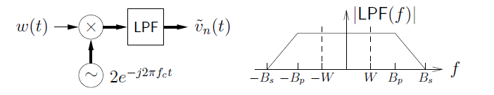
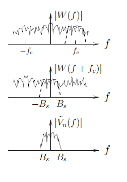
From the diagram,
is a baseband version of the bandpass noise
spectrum that occupies the frequency range
.
Since
is complex-valued,
is
non-symmetric.
Say that is real-valued white noise with power spectral density (PSD) . Since is constant over all f , the PSD of the complex noise will be constant over the LPF passband, i.e., :
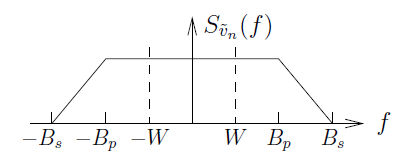
A well-designed communications receiver will suppress all energy outside the signal bandwidth W , since it is purely noise. Given that the noise spectrum outside will get totally suppressed, it doesn't matter how we model it! Thus, we choose to replace the lowpass complex noise with something simpler to describe: white complex noise with PSD :

We'll refer to as " complex baseband equivalent " noise.
Putting the signal and noise paths together, we arrive at the complex baseband equivalent channel model :
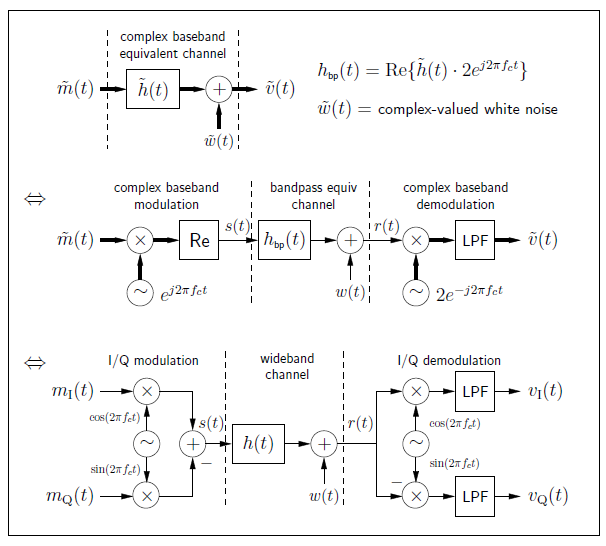
The diagrams above should convince you of the utility of the complex-baseband representation in simplifying the system model!
Notification Switch
Would you like to follow the 'Introduction to analog and digital communications' conversation and receive update notifications?

|
|

|
|

|
|

|
|

|
|

|
|

|
|

|
|

|
|

|