0.4 Linear programming: a geometric approach

We start by choosing our variables.

Let $x=\text{The number of hours per week Niki will work at Job I}\text{.}$

and $y=\text{The number of hours per week Niki will work at Job II}\text{.}$

Now we write the objective function. Since Niki gets paid $40 an hour at Job I, and $30 an hour at Job II, her total income I is given by the following equation.

Our next task is to find the constraints. The second sentence in the problem states, "She never wants to work more than a total of 12 hours a week." This translates into the following constraint:

The third sentence states, "For every hour she works at Job I, she needs 2 hours of preparation time, and for every hour she works at Job II, she needs one hour of preparation time, and she cannot spend more than 16 hours for preparation." The translation follows.

The fact that $x$ and $y$ can never be negative is represented by the following two constraints:

$x\ge 0$ , and $y\ge 0$ .

Well, good news! We have formulated the problem. We restate it as

Maximize $I=\text{40}x+\text{30}y$

Subject to:

In order to solve the problem, we graph the constraints as follows.

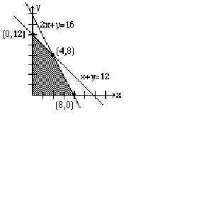
Observe that we have shaded the region where all conditions are satisfied. This region is called the feasibility region or the feasibility polygon.

The Fundamental Theorem of Linear Programming states that the maximum (or minimum) value of the objective function always takes place at the vertices of the feasibility region.

Therefore, we will identify all the vertices of the feasibility region. We call these points critical points. They are listed as (0, 0), (0, 12), (4, 8), (8, 0). To maximize Niki's income, we will substitute these points in the objective function to see which point gives us the highest income per week. We list the results below.

Clearly, the point (4, 8) gives the most profit: $400.

Therefore, we conclude that Niki should work 4 hours at Job I, and 8 hours at Job II.