<< Chapter < Page Chapter >> Page >
This module describes basic analog modulation techniques, including amplitude modulation (AM) with suppressed carrier, AM with a pilot tone or carrier tone, quadrature AM (QAM), vestigial sideband modulation (VSB), and frequency modulation (FM). Various demodulation techniques are also discussed, including envelope detection and the discriminator. Application examples include NTSC television and FM radio (both mono and stereo).
  1. Amplitude modulation (AM)
  2. Quadrature amplitude modulation (QAM)
  3. Vestigial sideband modulation (VSB)
  4. Frequency modulation (FM)

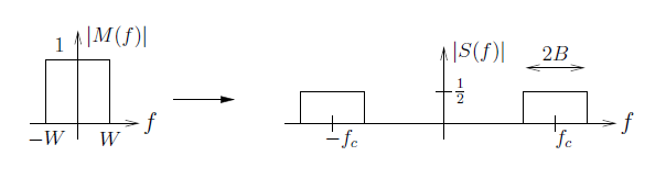
Am with “suppressed carrier”

AM of real-valued message m ( t ) (e.g., music) is

This figure contains one flowchart and two expressions. The flowchart begins with the variable m(t) with an arrow pointing to the right at a circle labeled x. Below the circle is a circle containing a tilde, labeled cos(2πf_ct). An arrow from the tilde circle points up at the x circle. To the right of the x circle is an arrow pointing to the right at the variable s(t). To the right of this flowchart are two expressions. The first reads s(t) = m(t)cost(2πf_ct). The second reads f_c = carrier freq. This figure contains one flowchart and two expressions. The flowchart begins with the variable m(t) with an arrow pointing to the right at a circle labeled x. Below the circle is a circle containing a tilde, labeled cos(2πf_ct). An arrow from the tilde circle points up at the x circle. To the right of the x circle is an arrow pointing to the right at the variable s(t). To the right of this flowchart are two expressions. The first reads s(t) = m(t)cost(2πf_ct). The second reads f_c = carrier freq.

Euler's cos ( 2 π f c t ) = 1 2 e j 2 π f c t + e - j 2 π f c t then implies

S ( f ) = - m ( t ) cos ( 2 π f c t ) e - j 2 π f t d t = 1 2 - m ( t ) e - j 2 π ( f - f c ) t d t + 1 2 - m ( t ) e - j 2 π ( f + f c ) t d t = 1 2 M ( f - f c ) + 1 2 M ( f + f c ) .
This figure contains two graphs. The first plots f on the horizontal axis, and |M(f)| on the vertical axis. There is a box of height 1 and width 2W on this graph. The base of the box sits on the horizontal axis, with the left side at value -W and the right side at W. To the right of this graph is an arrow pointing to the right at the second graph, which plots horizontal axis f against vertical axis |S(f)|. In the graph, there are two boxes, one centered on the horizontal axis at -f_c and the other centered at f_c. The width of these is measured as 2B. The height is measured as 1/2. This figure contains two graphs. The first plots f on the horizontal axis, and |M(f)| on the vertical axis. There is a box of height 1 and width 2W on this graph. The base of the box sits on the horizontal axis, with the left side at value -W and the right side at W. To the right of this graph is an arrow pointing to the right at the second graph, which plots horizontal axis f against vertical axis |S(f)|. In the graph, there are two boxes, one centered on the horizontal axis at -f_c and the other centered at f_c. The width of these is measured as 2B. The height is measured as 1/2.

Because m ( t ) R , know | M ( f ) | symmetric around f = 0 , implying the AM transmitted spectrum below f c is redundant! This motivates the QAM and VSB modulation schemes...
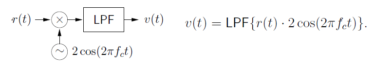
With f c known, AM demodulation can be accomplished by:

This figure contains one flowchart and two expressions. The flowchart begins with the variable r(t) with an arrow pointing to the right at a circle labeled x. Below the circle is a circle containing a tilde, labeled cos(2πf_ct). An arrow from the tilde circle points up at the x circle. To the right of the x circle is an arrow pointing to the right at a box labeled LPF. To the right is an arrow pointing to the right at the expression v(t). To the right of this flowchart is the expression v(t) = LPF{r(t)*2cos(2πf_ct)} This figure contains one flowchart and two expressions. The flowchart begins with the variable r(t) with an arrow pointing to the right at a circle labeled x. Below the circle is a circle containing a tilde, labeled cos(2πf_ct). An arrow from the tilde circle points up at the x circle. To the right of the x circle is an arrow pointing to the right at a box labeled LPF. To the right is an arrow pointing to the right at the expression v(t). To the right of this flowchart is the expression v(t) = LPF{r(t)*2cos(2πf_ct)}

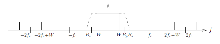
For a trivial noiseless channel, we have r ( t ) = s ( t ) , so that

v ( t ) = LPF { s ( t ) · 2 cos ( 2 π f c t ) } = LPF { m ( t ) · 2 cos 2 ( 2 π f c t ) 1 + cos ( 2 π · 2 f c t ) } = LPF { m ( t ) + m ( t ) cos ( 2 π · 2 f c t ) } = m ( t ) ,

assuming a LPF with passband cutoff B p W Hz and stopband cutoff B s 2 f c - W Hz:

This figure is a wide graph with horizontal axis f of three shapes and two dashed lines. In the middle of the graph, centered at the vertical axis and the origin, is a box  stretching from horizontal value -W to W. From the top of this box are two dashed lines that first start out horizontally and then decrease diagonally to the horizontal axis. The diagonal dashed lines land on horizontal values -B_s and B_s. Further outside are hash marks on either side of the dashed line, labeled -f_c and f_c. Beyond these are two more boxes, with bases on the horizontal axis. The inside corner of the boxes are labeled -2f_c + W and 2f_c - W, and the midpoints of the boxes are labeled -2f_c and 2f_c. Their height is not labeled but is approximately one-half the height of the box in the middle. This figure is a wide graph with horizontal axis f of three shapes and two dashed lines. In the middle of the graph, centered at the vertical axis and the origin, is a box  stretching from horizontal value -W to W. From the top of this box are two dashed lines that first start out horizontally and then decrease diagonally to the horizontal axis. The diagonal dashed lines land on horizontal values -B_s and B_s. Further outside are hash marks on either side of the dashed line, labeled -f_c and f_c. Beyond these are two more boxes, with bases on the horizontal axis. The inside corner of the boxes are labeled -2f_c + W and 2f_c - W, and the midpoints of the boxes are labeled -2f_c and 2f_c. Their height is not labeled but is approximately one-half the height of the box in the middle.

Note that we've assumed perfectly synchronized oscillators!

When the receiver oscillator has {freq,phase} offset { γ , φ } :

v ( t ) = LPF m ( t ) cos ( 2 π f c t ) · 2 cos ( 2 π ( f c + γ ) t + φ ) cos ( 2 π γ t + φ ) + cos ( 2 π ( 2 f c + γ ) t + φ ) = m ( t ) cos ( 2 π γ t + φ ) time-varying attenuation! .
a freq offset of λ = ν f c c Hz can occur when there is relative velocity of ν m/s between transmitter and receiver.

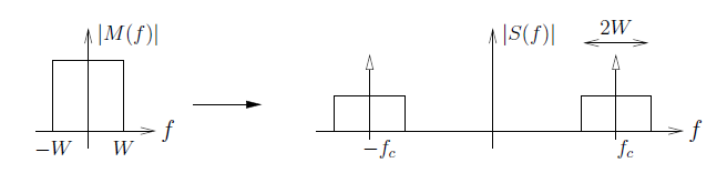
Am with “pilot tone” or “carrier tone”

It's common to include a pilot/carrier tone with frequency| f c :

s ( t ) = m ( t ) cos ( 2 π f c t ) + A cos ( 2 π f c t ) pilot/carrier tone = [ m ( t ) + A ] cos ( 2 π f c t ) S ( f ) = 1 2 M ( f - f c ) + M ( f + f c ) + A δ ( f - f c ) + A δ ( f + f c )
This figure is comprised of two cartesian graphs. The graph on the left is rather small, plotting f on the horizontal axis and |M(f)| on the vertical axis. The graph contains one large rectangle, with base sitting on the horizontal axis, and with measured to be from -W to W. To the right of this graph is an arrow pointing to the right at a larger graph, also plotting f on the horizontal axis, but this time with a vertical axis |S(f)|. In this graph there are two rectangles, each approximately one-half the height of the rectangle in the first graph, but with a similar width. The bases are both on the horizontal axis, and the centers of the bases are labeled -f_c and f_c. The width of each of these is measured with an arrow above, labeled 2W. In the center of the bases of these rectangles are vertical arrows that begin below the horizontal axis and point directly up. This figure is comprised of two cartesian graphs. The graph on the left is rather small, plotting f on the horizontal axis and |M(f)| on the vertical axis. The graph contains one large rectangle, with base sitting on the horizontal axis, and with measured to be from -W to W. To the right of this graph is an arrow pointing to the right at a larger graph, also plotting f on the horizontal axis, but this time with a vertical axis |S(f)|. In this graph there are two rectangles, each approximately one-half the height of the rectangle in the first graph, but with a similar width. The bases are both on the horizontal axis, and the centers of the bases are labeled -f_c and f_c. The width of each of these is measured with an arrow above, labeled 2W. In the center of the bases of these rectangles are vertical arrows that begin below the horizontal axis and point directly up.

Advantage: aids receiver with carrier synchronization.

Disadvantage: consumes transmission power.

While modern systems choose A max | m ( t ) | , many older systems use A > max | m ( t ) | , 
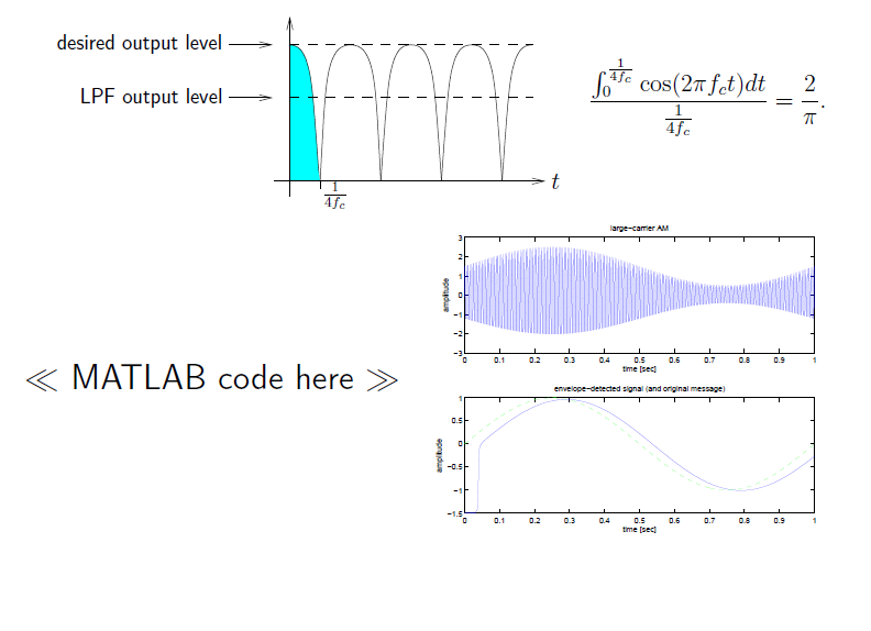
known as “large carrier AM,” allowing reception based on envelope detection :

v ( t ) = π 2 LPF { | r ( t ) | } - A m ( t ) (with a trivial channel)

where | · | can be easily implemented using a diode.

The gain π 2 above makes up for the loss incurred when LPFing the rectified signal:

This figure is comprised of three graphs, one equation, and one statement. Beginning in the top-left is a graph plotting t on the horizontal axis. There are a series of peaks in the first quadrant of the graph, with a peak beginning on the vertical axis and continuing downward. The first peak is shaded tea. The point where the first peak reaches the horizontal axis is measured at a horizontal value 1/4f_c. Midway up the vertical axis is a horizontal dashed line labeled LPF output level. Along the peaks is another dashed horizontal line labeled desired output level. There are three complete peaks, one half-peak at the beginning, and one half-peak at the end. To the right of the graph is an equation. The equation begins with a large fraction on the top, the numerator being the integral of lower bound 0 and upper bound 1/4f_c of cosine (2 pi f_c t) dt, and the denominator 1/4f_c. This is equal to 2 / pi. Below this equation on the right side are two graphs, the first plotting time against amplitude and showing closely packed waves moving together with increasing, then decreasing, then increasing amplitudes. The graph is titled large-carrier AM. The second plots time against amplitude and contains two graphs that closely follow one another with a simple wave and is titled envelope-detected signal (and original message). To the left of these graphs is the statement MATLAB code here. This figure is comprised of three graphs, one equation, and one statement. Beginning in the top-left is a graph plotting t on the horizontal axis. There are a series of peaks in the first quadrant of the graph, with a peak beginning on the vertical axis and continuing downward. The first peak is shaded tea. The point where the first peak reaches the horizontal axis is measured at a horizontal value 1/4f_c. Midway up the vertical axis is a horizontal dashed line labeled LPF output level. Along the peaks is another dashed horizontal line labeled desired output level. There are three complete peaks, one half-peak at the beginning, and one half-peak at the end. To the right of the graph is an equation. The equation begins with a large fraction on the top, the numerator being the integral of lower bound 0 and upper bound 1/4f_c of cosine (2 pi f_c t) dt, and the denominator 1/4f_c. This is equal to 2 / pi. Below this equation on the right side are two graphs, the first plotting time against amplitude and showing closely packed waves moving together with increasing, then decreasing, then increasing amplitudes. The graph is titled large-carrier AM. The second plots time against amplitude and contains two graphs that closely follow one another with a simple wave and is titled envelope-detected signal (and original message). To the left of these graphs is the statement MATLAB code here.

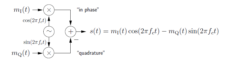
Quadrature amplitude modulation (qam)

QAM is motivated by unwanted redundancy in the AM spectrum, which was symmetric around f c .

QAM sends two real-valued signals { m I ( t ) , m Q ( t ) } simultaneously, resulting in a non-symmetric spectrum.

This figure is a flowchart, beginning with an expression m_I(t), with an arrow pointing to the right at a circle containing an x. Below this is the expression m_Q(t), with an arrow pointing to the right at another circle containing an x. In between these two circles is a circle containing a tilde, with an arrow pointing up and another arrow pointing down at the two x-circles. These two arrows are labeled cos(2 pi f_c t) for the one pointing up, and sin (2 pi f_c t) for the one pointing down. To the right of both of the x-circles are arrows pointing at a single circle containing a plus sign, with the lower arrow labeled with a minus sign. The lower arrow is labeled quadrature, and the upper is labeled in phase. To the right of this plus-circle is an arrow pointing to the right at a large equation that reads s(t) = m_I(t)cos( 2 pi f_c t) - m_Q(t)sin (2 pi f_c t). This figure is a flowchart, beginning with an expression m_I(t), with an arrow pointing to the right at a circle containing an x. Below this is the expression m_Q(t), with an arrow pointing to the right at another circle containing an x. In between these two circles is a circle containing a tilde, with an arrow pointing up and another arrow pointing down at the two x-circles. These two arrows are labeled cos(2 pi f_c t) for the one pointing up, and sin (2 pi f_c t) for the one pointing down. To the right of both of the x-circles are arrows pointing at a single circle containing a plus sign, with the lower arrow labeled with a minus sign. The lower arrow is labeled quadrature, and the upper is labeled in phase. To the right of this plus-circle is an arrow pointing to the right at a large equation that reads s(t) = m_I(t)cos( 2 pi f_c t) - m_Q(t)sin (2 pi f_c t).

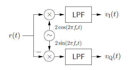
QAM demodulation is accomplished by:

This is a flowchart that starts with the expression r(t). From r(t) there are two arrows pointing at two separate circles containing an x, above and below one another. The arrow that points to the lower circle is labeled with a minus sign. In between the two circles is another circle with a tilde. Above and below this circle are arrows pointing up and down at the x-circles, and the arrows are labeled 2 cosine (2 pi f_c t) above  and 2 sine (2 pi f_c t) below. To the right of the x-circles are two boxes labeled LPF. To the right of these boxes are two arrows pointing to the right at two final expressions, v_I(t) above and v_Q(t) below. This is a flowchart that starts with the expression r(t). From r(t) there are two arrows pointing at two separate circles containing an x, above and below one another. The arrow that points to the lower circle is labeled with a minus sign. In between the two circles is another circle with a tilde. Above and below this circle are arrows pointing up and down at the x-circles, and the arrows are labeled 2 cosine (2 pi f_c t) above  and 2 sine (2 pi f_c t) below. To the right of the x-circles are two boxes labeled LPF. To the right of these boxes are two arrows pointing to the right at two final expressions, v_I(t) above and v_Q(t) below.

where the LPF specs are the same as in AM, i.e., passband edge B p W Hz and stopband edge B s 2 f c - W Hz.

For a trivial channel, we have r ( t ) = s ( t ) , so that

v I ( t ) = LPF { r ( t ) · 2 cos ( 2 π f c t ) } = LPF { m I ( t ) 2 cos 2 ( 2 π f c t ) 1 + cos ( 4 π f c t ) - m Q ( t ) 2 sin ( 2 π f c t ) cos ( 2 π f c t ) sin ( 4 π f c t ) } = m I ( t ) v Q ( t ) = LPF { - r ( t ) · 2 sin ( 2 π f c t ) } = LPF { - m I ( t ) 2 cos ( 2 π f c t ) sin ( 2 π f c t ) sin ( 4 π f c t ) + m Q ( t ) 2 sin 2 ( 2 π f c t ) 1 - cos ( 4 π f c t ) } = m Q ( t ) ,

assuming synchronized oscillators.

When the oscillators are not synchronized, one gets coupling between the I&Q components as well as attenuation of each. Writing the I&Q signals in the “complex-baseband” form

Get Jobilize Job Search Mobile App in your pocket Now!

Get it on Google Play Download on the App Store Now


Source:  OpenStax, Introduction to analog and digital communications. OpenStax CNX. Sep 14, 2009 Download for free at http://cnx.org/content/col10968/1.2
Google Play and the Google Play logo are trademarks of Google Inc.

Notification Switch

Would you like to follow the 'Introduction to analog and digital communications' conversation and receive update notifications?

Ask