0.3 The kinematics of fluid motion  (Page 4/9)

from which it follows that $u\delta y-v\delta x$ is an exact differential, equal to $\delta \psi$ say. Then

and the unknown scalar function $\psi (x,y,t)$ is defined by

where ${\psi }_o$ is a constant and the line integral is taken along an arbitrary curve joining some reference point O to the point $P$ with co-ordinates $x$ , $y$ . In this way we have used the mass-conservation equation to replace the two dependent variables $u$ , $v$ by the single dependent variable $\psi$ , which is a very valuable simplification in many cases of two-dimensional flow.

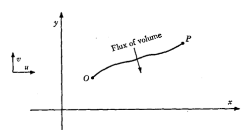
The physical content of the above argument also proves to be of interest. The flux of fluid volume across a curve joining the points 0 and $P$ in the ( $x$ , $y$ )-plane (by which is meant the flux across the open surface swept out by translating this curve through unit distance in the $z$ -direction), the flux being reckoned positive when it is in the anti-clockwise sense about $P$ , is given exactly by the right-hand side of (2.2.8) (see figure 2.2.1). Now the flux of volume across the closed curve formed from any two different paths joining 0 to $P$ is necessarily zero when the region between the two paths is wholly occupied by incompressible flow. The flux represented by the integral in (2.2.8) is therefore independent of the choice of the path joining $O$ to $P$ , provided it is one of a set of paths of which any two enclose only incompressible fluid, and therefore defines a function of the position of $P$ , which we have written as $\psi -{\psi }_o$ .

Since the flux of volume across any curve joining two points is equal to the difference between the values of $\psi$ at these two points, it follows that $\psi$ is constant along a streamline, as is also apparent from (2.2.7) and the equation (2.1.1) that defines the streamlines. $\psi$ is termed the stream function , and is associated (in this case of two-dimensional flow) with the name of Lagrange. The function can also be regarded as the only non-zero component of a 'vector potential' for $\mathbf{u}$ (analogous to the vector potential of the magnetic induction, which also is a solenoidal vector, in electromagnetic field theory), since (2.2.7) can be written as

It is common practice in fluid mechanics to provide a picture of a flow field by drawing various streamlines, and if these lines are chosen so that the two values of $\psi$ on every pair of neighboring streamlines differ by the same amount, $\epsilon$ say, the eye is able to perceive the way in which the velocity magnitude $q$ , as well as its direction, varies over the field, since

Examples of families of streamlines describing two-dimensional flow fields, with equal intervals in $\psi$ between all pairs of neighboring streamlines, will be found in figures 2.6.2 and 2.7.2.

Expressions for the velocity components parallel to any orthogonal coordinate lines in terms of $\psi$ may be obtained readily, either by the use of (2.2.9) or with the aid of the relation between $\psi$ and the volume flux 'between two points'. For flow referred to polar co-ordinates ( $r$ , $\theta$ ), we find, by evaluating the flux between pairs of neighboring points on the $r$ - and $\theta$ -co-ordinate lines and equating it to the corresponding increments in $\psi$ (allowance being made for the signs in the manner required by (2.2.8)), that